This chapter discusses the functions of the Tool Manager, which is the graphical user interface (GUI) that lets you specify data and configuration information for the MineSet tools in this package. It provides an overview of this interface, then describes every component of each panel that this interface displays for all MineSet tools.
 | Note: Any screens dedicated to a specific tool are discussed in the chapter for that tool; for example, the screen for specifying the Tree Visualizer's configuration file is discussed in Chapter 5, “Using the Tree Visualizer.” |
The Tool Manager is the initial graphical user interface (GUI) you use for most of your interactions with the MineSet components. With Tool Manager you can select an existing data source, transform or analyze that data, and visualize the results using any of the MineSet individual tools. You can step through the process in these sections:
| Note: The Tool Manager generally does not support data files not created by the Tool Manager without some manual work to make them compatible. |
You can specify the source of the data as being from a:
database table
database SQL query
file
Often the original data is unsuitable for mining or visualization. It may contain irrelevant or redundant columns, data types that are not applicable for viewing, or inconsistencies that result in unhelpful visualization. You can transform the data with the Tool Manager to display it in a useful form in any of these ways:
mining tools—finds patterns in data
binning variables—discretizes column values into groups, such as grouping years by decade
removing columns—excises unneeded columns to save space
adding new columns—creates columns that are functions of existing columns
aggregation—finds the average, sum, min, max, or counts of column values
filtering—selects a subset of the data based on an expression using column values
sampling—selects a random subset of the data
making arrays—takes the values of one column and turns them into an array indexed by discrete values in another column
distributing columns—makes two or more new columns from a single column of values, distributed by the discrete values of another column
The final step, having transformed the data, is to visualize the results.You can do this in any of these ways; for example you can display the data on the screen as:
a hierarchy (Tree Visualizer—Option, Decision, Regression)
a map (Map Visualizer)
a scatter plot showing relations of numerous independent variables (Scatter Visualizer and Splat Visualizer)
as associated rules (Rules Visualizer)
as evidence and probability (Evidence Visualizer)
as box plots and histograms (Statistics Visualizer and Cluster Visualizer)
as layered tables or cakes (Decision Table)
With Tool Manager you can map data values to specific visual elements on the screen such as:
colors
bars
heights
Finally, Tool Manager lets you control those options not related to data, including:
background colors
grid spacing
label sizes
You can run the Tool Manager in two modes:
interactive mode—the Tool Manager provides windows, menus, buttons, and so on, to let you access, mine, and visualize your data. Interactive mode also lets you save a description of your actions to a “session file” for future use.
batch mode—the Tool Manager performs all the actions described in a session file without bringing up windows. For example, batch mode is useful for lengthy computations that need to be done every night, so that the data can be fully prepared each morning.
There are three ways to start the Tool Manager in interactive mode:
Double-click the MineSet icon, which is in the Applications or the MineSet page of the icon catalog. The Tool Manager starts with the same configuration used in the last Tool Manager session.
Double-click an icon representing a session file saved from a previous invocation of the Tool Manager. This starts the Tool Manager with that session file.
Start the Tool Manager from the UNIX shell command line by entering this command at the prompt:
mineset [ sessionFile ]
Here, sessionFile is optional and specifies the name of the session file to use. If you do not specify a configuration file, MineSet starts up with the configuration most recently used.
To start the Tool Manager in batch mode, enter this command at the UNIX shell prompt:
mineset_batch [-s serverPassword -d databasePassword] sessionFile |
The -s and -d options allow you to specify the password for logging into the server and database respectively. If you do not specify these options, mineset_batch will ask you to type in the passwords, thus these options are useful when running mineset_batch from a shell script. To specify that there is no password for either the server or database, use -s or -d followed by two double quotes, that is,
mineset_batch -s "" -d "" foo.mineset |
If you specify one of the two passwords, you must specify both.
Figure 3-1 shows the Tool Manager's startup window.

This window consists of two panels related to the specific dataset and tool chosen, and two information sections. Specification of servers and data sources is done via popup dialogs accessible from the File menu.
The panels and information sections are
Data Transformations, which lets you modify the data from your data source.
Data Destination, which lets you create visualizations based on your data, save the data to a file, mine the data for association rules, create classifiers based on the data, or find important columns in the data.
The top panel, which provides information on the currently selected data source.
The bottom panel, which contains a stream of information on the status on certain operations.
The following sections describe each panel of the main Tool Manager window.
Data sources are selected using the first set of menu items in the File menu.
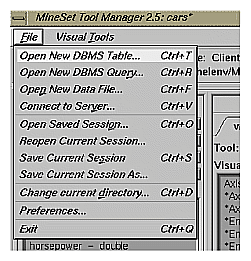
The first three options in the File menu let you select the data source from a
DBMS Table
DBMS Query
Data File
The fourth option, Connect to Server, lets you connect to a server without specifying the data source.
You must connect to a server to get information from a database or mining tool, or to apply transformations to an existing data file. It is not necessary if you plan to visualize an existing client data file without transforming it.
Use the Open New Data File menu option to work with an existing data file. When you select this option, the dialog in Figure 3-3 appears.
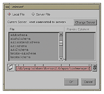
This dialog box, which is similar to a standard file selection dialog box, provides a toggle at the top to select client versus server files; it also has a label indicating the name of the current MineSet server, and a push button to let you log in to a new server. The radio buttons at the top let you select files on your client machine (in any directory accessible to you) or files that exist in your single cache on the DataMover server, (see “Configuring the DataMover Server” in Chapter 2.)
When you select the name of a file from the list in the left window, the columns of that data file are shown in the right window.
When you click the Change Server button, a dialog prompts you for a server name, login name, and password to connect to the server (see Figure 3-5).
If you want to access a data file created outside of Tool Manager, you must create a .schema file for it. This is a text file containing a configuration “input” section, which gives the name of the data file and describes its layout. The Tool Manager supports input sections similar to those for the Tree Visualizer (described in Appendix B), except that it does not support variable length arrays or the monitor option.
Use the Open New DBMS Table menu option to work with tables in a DBMS. Selecting this option causes the dialog box in Figure 3-4 to be displayed.
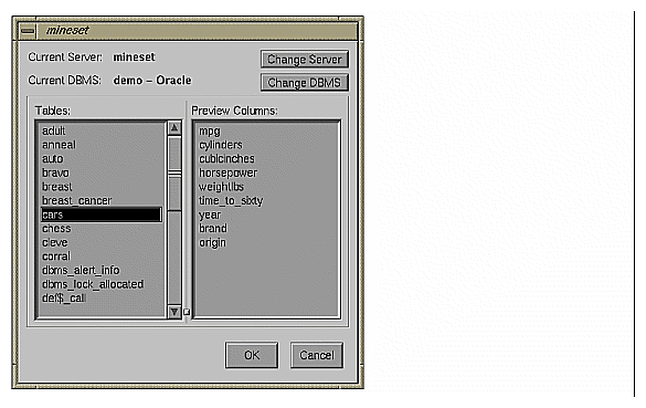
The name of the currently selected server appears to the left of the Change Server button. If you click this button, the dialog box shown in Figure 3-5 appears. This lets you specify a server name, login, and password.
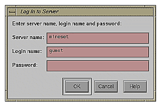
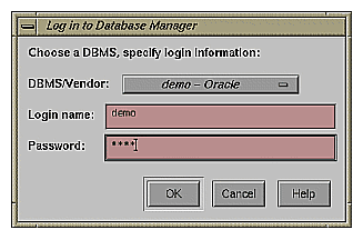
Once you have logged in to a server, click the Change DBMS button to bring up a dialog box that contains a popup menu listing DBMS names/vendors (see Figure 3-6). Select a DBMS from the menu, and enter the login name and password to connect to the DBMS. Note that the DBMS login and password are usually different from those required to connect to the server.
If you have logged on to an Oracle DBMS, the dialog box appears as shown in Figure 3-4, with a list of tables on the left. When you select a table, the columns for that table are shown on the right.
If the DBMS is Informix or Sybase, the dialog box shown in Figure 3-7 appears, with a list of databases for the DBMS. Select a database, and the list of tables in that database are shown.
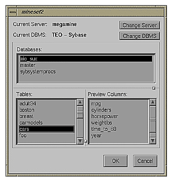
To use a certain table in the Tool Manager, select the table you want to use and click OK.
Use the Open New DBMS Query menu option to work with tables created via SQL queries against a DBMS. Selecting this option causes the dialog box in Figure 3-8 to appear.
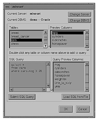
Selecting a server and DBMS in this dialog box has the same effect as selecting those items in the Open New DBMS Table dialog box.
The SQL query is shown in the panel at the lower left. You can enter the query there, or load it from a disk file using the Load SQL from File button. The names of tables and columns in the current DBMS are shown to help build queries. To have their names transferred to the SQL query panel, double-click on them.
When you have entered the SQL query, click the Submit SQL Query button to send it to the DBMS for execution. The table columns resulting from the query appears on the right.
The Data Transformations panel lets you manipulate the tables with which you want to work. After you have selected a table (via the File menu, described above), its column headings appear in the Current Columns window of the Data Transformations panel (Figure 3-9).
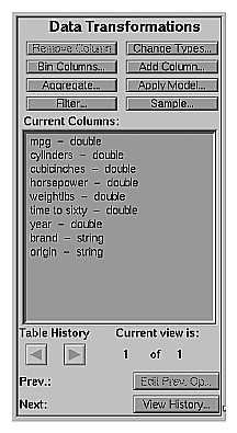
The functions of the displayed options are:
Remove Column—lets you delete one or more columns that are not relevant to the current visualization or mining.
Bin Columns—lets you assign each record to a group that falls within a certain range (bin) of column values. For example, an age column may be binned into the ranges (bins): 0-18, 19-25, 26-35, and so on.
Aggregate—adds columns of records (sum), creates a new column representing maximum or minimum values, or makes an array from a column that is indexed by other columns.
Filter—lets you select a subset of the data based on an expression involving column values, for example, leave only those records in which the age is less than 20.
Change Types—lets you change a column's name as well as its type.
Add Column—lets you add a new column based on a mathematical expression. For example, add a column “minor” based on the column “age,” using the expression: “if age is less than or equal to 18 then minor is true; else minor is false.”
Apply Model—lets you use a previously created classifier to label new records, to estimate probabilities for label values, to test the classifier on new data, or to backfit data to an existing classifier (see Chapter 10, “MineSet Inducers and Classifiers,” for details).
Sample—lets you select a random subset of the data. This is useful for very large data sets.
Remove Column lets you delete columns by selecting the column name or names in the Current Columns panel, then clicking this button. The items in the Current Columns panel change to show the new table columns. To choose multiple contiguous columns for simultaneous removal, click and drag the mouse over the columns. To choose multiple non-contiguous columns for simultaneous removal, hold down the Ctrl key while selecting the additional columns.
Binning lets you sort the information from one or more columns into groups in a new column or columns (for example, with a range of ages, 0-18, 19-25, 26-35, and so on). Click Bin Columns to get a dialog box that lets you specify the binning options (Figure 3-10).
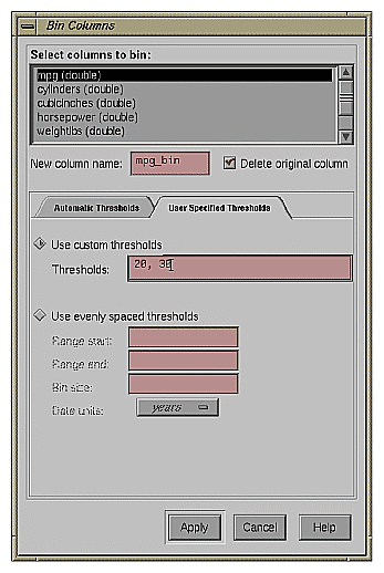
This dialog box lets you
choose the column that is to be divided into bins
specify the name of the new column to contain values for the bins
set bin thresholds, or specify a range with thresholds at regular intervals
To specify binning options for one or more columns, select the column name(s), choose the appropriate options below, and click the Apply button at the bottom of the dialog box.
If you select only one column for binning, the name of the resulting binned column appears in the “New column name” box, and you can type in a new name if you like. In the example shown in Figure 3-10, mpg_bin is the name for the new column; in this case, it provides a range of fuel efficiencies. If you select more than one column for binning, New column name stays inactive.
Next to New column name is a check box labeled “Delete original column”. When chosen, this option automatically deletes the original column after binning. Click the check box to turn this function on or off.
In the middle of the Bin columns dialogue box are two tabs for choosing Automatic Thresholds or User Specified Thresholds. Choose Automatic Thresholds if you'd like the computer to suggest the bins or User Specified Thresholds if you'd like to specify the thresholds yourself.
If you've chosen the Automatic Thresholds tab, the program can use machine learning to suggest bins.
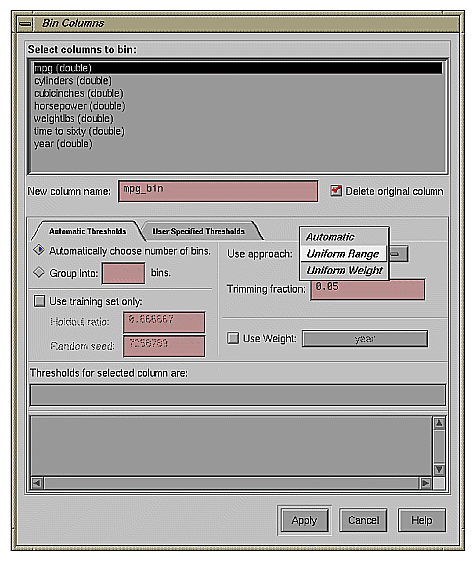
The first choice under Automatic Thresholds is between the Automatically choose number of bins and the Group into: ___ bins buttons. Click Automatically choose number of bins to let the computer decide the best number of bins. If you choose to specify the number of bins, click Group into: ___ bins, and type the number of bins you want into the field.
There are three ways to categorize data into bins:
Automatic—you must also select a discrete label. The thresholds are chosen so that the distributions of labels within different bins are as different as possible. This approach continues to create thresholds that split the range until no additional interval is considered significant.
The “Min weight per bin” text field lets you specify the minimum weight in any bin; this prevents the creation of bins with less weight than the number specified. No interval is split if the two resulting subintervals do not each contain at least the minimum weight you specify. By default, each instance has unit weight. In this situation, specifying the Min weight per bin is the same as specifying the minimum number of instances per bin.
Rather than specifying the minimum weight per bin, it is possible to have the algorithm set that value automatically. The check box labeled Auto causes the algorithm to calculate a value for the minimum weight per bin based on the total weight of the instances: the more total weight, the higher the minimum weight per bin (the relationship is logarithmic).
Uniform Range—the algorithm divides the value range into the specified number of uniformly sized subintervals. The upper and lower bounds for the extreme ranges include any values outside the ranges observed in the data. For example, if the values for an attribute are in the range 3-8, and you specify four bins, the thresholds identified are 4.25, 5.5 and 6.75, corresponding to the ranges:
≤ 4.25
> 4.25 to 5.5
> 5.5 to 6.75
> 6.75
Uniform Weight—the algorithm divides the value range into the specified number of equal weight bins. Unlike Uniform Range, in which thresholds are identified that separate the value range into intervals of equal size, Uniform Weight identifies thresholds that group the instances into subsets of equal weight. By default, each instance has unit weight. In this case, the Uniform Weight approach produces the specified number of bins, each containing an approximately equal number of instances.
Both Uniform Range and Uniform Weight let you specify a trimming fraction, which indicates the fraction of extreme values to be excluded from the value range prior to generating bins. The default trimming fraction is 0.05. This excludes the 5% of the instances with the most extreme values (2.5% with the lowest values in the range, and 2.5% with the highest values in the range). Trimming tends to reduce the influence of outliers on the generation of thresholds.
All of the approaches let you decide whether you want to specify the number of bins or let the algorithm select the number automatically. For the Uniform Range and Uniform Weight approaches, the automatic selection of the bins is based on the number of distinct values: the more distinct values, the more bins are chosen (the relationship is logarithmic).
Typically, all of the available instances are used when identifying thresholds. When binned attributes are later used to induce a classifier, the error estimates for that classifier tend to be overly optimistic. This is because distributional information from the test set was used to identify thresholds. Use training set only prevents the binning approaches from looking at the records in the test set when identifying thresholds. This tends to give a more realistic estimate of the classifiers' error rate. Use training set only requires the user to specify the same Holdout ratio and Random seed (see “Error Options for Inducers” in Chapter 10) that are used to create the holdout set for estimating classifier error.
The Use Weight menu lets you weight the instances by any numeric attribute. Changing instance weight affects both Automatic and Uniform Weight, but has no affect on the Uniform Range.
If you click Apply, the Tool Manager picks bin thresholds and displays them in the “Thresholds for selected column are” text field. The text field at the bottom of the Bin Columns window shows the progress of the binning algorithm and any errors that occur.
If you specify your own thresholds (as shown in Figure 3-10), you can choose between Use custom thresholds or Use evenly spaced thresholds by clicking either button. When you type in the thresholds, you must click Apply to make those thresholds effective for the selected columns.
The Use custom thresholds text box lets you enter the range criteria. For example, you could enter the numbers 18, 30, 50, 60. This results in the following ranges: 0-18, 19-30, 31-50, 51-60, 61+. Note that you enter only the digits and commas, not the ranges.
To specify equally spaced bins over a range of values, click the Equally Spaced Bins button. This activates the three text fields below it. You can type the start of the binning range, the end of the range, and the spacing of the bins, respectively, into these fields. If you are binning a column that is a date, you can specify units of time for the bin spacing (using the “Date units” popup menu under the text fields). This would permit you, for example, to bin a time period into bins of three weeks. Dates entered into these fields must be typed in the form “MM/DD/YY”. Possible time units are as follows:
years
quarters
months
days
hours
minutes
seconds
The Use custom thresholds text box accepts dates either in double quotes (as shown below), or without. If you enter dates without quotes, the quotes are added automatically.
"1/1/96", "2/1/96", "3/1/96", "4/1/96", "5/1/96", "6/1/96"
However, do not put quotes around dates used with Use evenly spaced thresholds.
Before describing the features and effects of the Aggregate button (see page 86), this section provides an introduction to the concept of arrays and distribution as used in the aggregation feature.
The Aggregate button lets you perform simple aggregations (for example, sum, min, max, and so on), make arrays, and distribute columns. (See Table 3-1)
Table 3-1. Aggregate Example 1
State | Age_bin | Total $ Spent |
|---|---|---|
CA | 0-20 | $50 |
CA | 21-40 | $454 |
CA | 41-60 | $693 |
NY | 0-20 | $35 |
NY | 21-40 | $541 |
NY | 41-60 | $628 |
If you make Total $ Spent into an array indexed by the binned column Age_bin, the resulting table has only two columns:
Table 3-2. Aggregate Example 2
State | Total $ Spent [Age_bin] |
|---|---|
CA | [$50, $454, $693] |
NY | [$35, $541, $628] |
In this case, making an array reduces the number of columns by one, and also reduces the number of rows by four. Arrays are useful for the Tree Visualizer tool; they are necessary if you want to use sliders in Scatter Visualizer and Map Visualizer displays.
Distributing columns is similar, but different in several important ways. Instead of producing a single new column holding many values, distributing produces one new column for each value of the index. For example, if in the first table was not made an array, but instead distributed by Age_bin, the result is:
Table 3-3. Aggregate Example 3
State | Total $_0-20 | Total $_21-40 | Total $_41-60 |
|---|---|---|---|
CA | $50 | $454 | $693 |
NY | $35 | $541 | $628 |
Thus, distributing increases the number of columns but decreases the number of rows.
If you have more than one binned column (for example, Age_bin and Sex_bin), you can make a two-dimensional array (indexed by combinations of Age_bin and Sex_bin). You also can distribute and make an array at the same time.
This table has two binned columns: one for age, one for sex.:
State | Age_bin | Sex_bin | Total $ Spent |
|---|---|---|---|
CA | 0-20 | 1 | $20 |
CA | 0-20 | 2 | $30 |
CA | 21-40 | 1 | $220 |
CA | 21-40 | 2 | $234 |
CA | 41-60 | 1 | $401 |
CA | 41-60 | 2 | $292 |
If you make Total $ Spent an array indexed by age, and remove Sex_bin, the results are:
Table 3-5. Results When Making Total $ Spent an Array
State | Total $ Spent [Age_bin] |
|---|---|
CA | [$50, $454, $693] |
If you do not remove Sex_bin, the results are:
Table 3-6. Results When Specifying Sex_bin
State | Sex_bin | Total $ Spent [Age_bin] |
|---|---|---|
CA | 1 | [$20, $220, $401] |
CA | 2 | [$30, $234, $292] |
If you make an array by both Age_bin and Sex_bin, the results are:
Table 3-7. Results of Making an Array by Age_bin and Sex_bin
State | Total $ Spent [Age_bin] [Sex_bin] |
|---|---|
CA | [$20, $220, $401, $30, $234, $292] |
Finally, if you distribute by Sex_bin and index by Age_bin, the results are:
Table 3-8. Results of Distributing Sex_bin and Indexing by Age_bin
State | Total $ Spent [Age_bin], Sex = 1 | Total $ Spent [Age_bin], Sex = 2 |
|---|---|---|
CA | [$20, $220, $401] | [$30, $234, $292] |
The examples above (with the exception of Table 3-5) had exactly one relevant value for each array element, and the distribution merely rearranged existing data values. For the example in Table 3-5, there were two data values for each array element, and these were summed. MineSet provides several aggregation options for datasets containing more than one value to be distributed into a given output array element. The most common option is to add the values (as done in Table 3-5). This is useful when accumulating expenditures into budgets, for example. You also can take the minimum, maximum, and average of the total number of values, as well as count them.
When distributing values for a given dataset, it is possible that there are no values appropriate for a particular bin. In this case, for min, max, avg, and sum aggregations, the DataMover fills in a value of NULL. For count aggregations, the DataMover fills in a value of 0.
You can use the Aggregate button to create simple aggregations, make arrays, or distribute columns. Clicking this button causes the Aggregate dialog box to appear (Figure 3-12). It shows three lists, with the columns in the current table appearing in the middle list. If you want to aggregate, distribute, or turn a column into an array, select the name of the column, and click the left arrow button between the left and center lists. Below are popup menus that let you specify indexes (if the result is to be an array) and a distribution column (if the result is to be distributed). In addition, at the bottom of the dialog box are five toggles that let you specify how different values are to be combined when aggregated: either summed, averaged, the min or max value, or the count. When you are aggregating number-valued columns, you can choose any combination of these options. For other types, only count is permitted. If you choose more than one option, you get more than one result. For example, selecting average and max gives you one result with average values, and another one holding the max values.
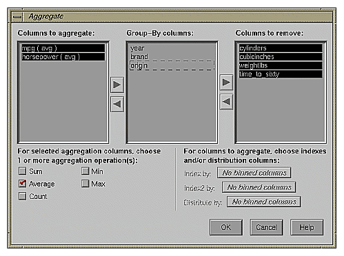
The three lists of column names are given below:
Group-By columns (the default); this keeps the columns unchanged throughout the operation. For each set of records with the same combination of values in the Group By columns, only one record is output in the resulting table, with values in the aggregated columns summed, averaged, minned, maxed, or counted (depending on the checkboxes at the bottom of the panel).
Columns to remove, as can be seen with the Sex_bin column in Table 3-5
After you have finished with the additional aggregate criteria dialog box, the Current Columns text box in the Table Processing window shows the new column names that result from applying these criteria.
This button lets you filter the data via a mathematical expression. The resulting table includes only records for which the expression is true (or, if numerical, non-zero). When you click Filter, the Filter dialog (Figure 3-13) appears.
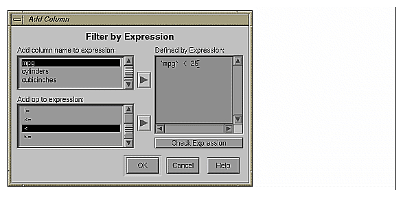
This dialog box lets you select column names and operators on the left to build an expression on the right. For a complete description of the expression definition language, see “The Configuration File” in Appendix B.
This button lets you change the name of a column, as well as its type.
Some databases store numerical values as strings. Oracle stores all numbers (both integers and real numbers) in a single format, which defaults to the data type double in the Tool Manager. You can use the Change Types button to ensure that these values are processed correctly. To change the type of one or more columns, click the Change Types button. A new dialog box appears (see Figure 3-14). This dialog box contains a window with a list of column headings and their respective types.
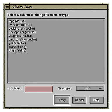
First select a column heading in the window. Then click the New type button. This produces a popup list of the possible types (invalid types are grayed out), as shown in Figure 3-15.
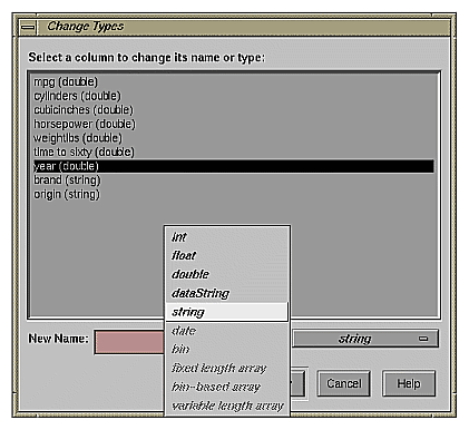
float—represents a single-precision floating-point number. The decimal point is optional when representing a floating-point number.
double—represents a double-precision floating-point number. The decimal point is optional when representing a floating-point number.
dataString—represents a string that is unlikely to appear multiple times. If it appears multiple times, several copies are made. A dataString can be used to store an address. Addresses are unlikely to be compared, and each record can have a different address.
string—represents a string of characters that can appear multiple times in the data file. Unlike a dataString, only a single copy of a given string is stored in memory, no matter how many times it appears in the data. This saves memory for strings appearing many times.
Comparing strings is also much quicker than comparing dataStrings. However, reading in strings can be slower than reading in dataStrings because it is necessary to look for duplications. An example of string use would be for a division name that appears once for each department in the division. If you are unsure whether to use a string or a dataString, use a string.
fixed-length array—an array of values of fixed size, not created by the Tool Manager.
bin-base array—an array of values as can be created by the Tool Manager.
variable-based array—an array of values of variable size, not created by the Tool Manager.
After selecting a new type, click Apply to have the change take effect.
If you try to convert an inappropriate field (such as a name) to a number, the resulting values are all zeroes.
| Note: When the data source is an existing file, there are fewer possibilities available for changing any given column. |
You can use the Add Column button to create a new column whose values are computed based on a mathematical expression. For example, you could add a new column whose values are the ratio of values from two existing columns. Click Add Column to get a dialog box that lets you specify the new column name and expression (Figure 3-16).
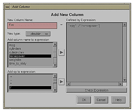
In the upper left of this dialog box is a field for entering the new column's name. Below this is a popup menu that lets you specify the column type (integer, string, floating point, and so on).
The right-hand side of the dialog contains a large text entry area where you can type in a definition of the expression (for a complete description of the expression definition language, see “The Configuration File” in Appendix B). As a shortcut to typing column names and operators, scrolled lists in the lower left of the dialog display all columns in the current table and all possible operators. To insert a column name or operator into the expression, either double-click it in its scrolled list, or select it and click the arrow button to the right of the scrolled list.
To check the expression you have created, click the Check Expression button. If there is an error, a dialog box appears, indicating what the error is and where it occurred. When you click OK, the expression is automatically checked, and the dialog box is not removed unless the expression is correct.
The Add Column dialog box checks for type compatibility: if you have assigned a numerical expression to a string column (or vice versa), a warning message appears, and the type of the new column is automatically changed to be correct.
The Apply Model button lets you use a previously created model to label new records in the current table, to estimate probabilities for a label value, to test the performance of the model on the current table, or to backfit the current table onto an existing model. See Chapter 10, “MineSet Inducers and Classifiers,” for details.
This button lets you select a random subset of the data. This is useful for data sets that are too large to work with efficiently. When you click Sample, the Sampling dialog box (Figure 3-17) appears.
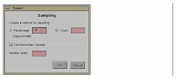
You can sample two ways: as a percentage of the current table, or by setting the maximum number of records to put in the sample. Percentage sampling is approximate, you can get slightly more or slightly fewer records than the exact percentage would indicate. The random sample is based on a numeric seed that can be specified in the sampling dialog. If no seed is specified, the number 1 is used as the seed. If you want a different random sample, specify a different random seed.
When you click the Complementary Sample toggle, you get all records except those that fall in the random sample. That is, if you get a 10% sample with the Complementary Sample not clicked, when you click it, you get the remaining 90% of the data.
Table processing is a series of operations performed by using the buttons described above. To allow you to see this series of steps, and go back if you made a mistake, there are two Table History buttons at the bottom of the Table Processing panel (Figure 3-18). When you click the left arrow button, the columns window shows the table as it appeared at an earlier step. Clicking the right arrow button returns the table to its current state.
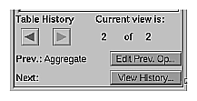
To the right of the history buttons is the information field Current view is, which counts the changes you've made and indicates which step you are viewing. The two integers in this field indicate which table view you're looking at, out of the total number of table views that exist. For example, if you've made two changes, you can view the original table (1 of 3), the table after the first change (2 of 3), or the table after the second change (3 of 3).
As you go back and forth using the Table History buttons to view earlier versions of the table, the Prev: and Next: fields (under the arrow buttons) help you keep track of where you are in the history of the table. For any table you view, the Prev: field tells you what the previous change was, and the Next: field tells you the next change.
The Edit Prev. Op. button allows you to edit the operation shown in the Prev. field. (This button is not active when Current view is: 1 of some number, because that is the original table, with no previous changes.) When you click the Edit Prev. Op. button, the dialog box for the previous operation comes up, and you can make changes to that operation. For example, if the previous operation was binning columns, when you click Edit Prev. Op., the Bin Columns dialog box appears.
Note that by changing a previous operation, you could affect operations you set up subsequent to the current one. For example, if you delete a column that you used in a subsequent binning operation, that binning operation becomes invalid. The Edit History button can help you avoid such problems.
When you click the View History button, the panels showing the current column and data destination are replaced by a panel showing you the complete history of the Data Transformation table (Figure 3-19). Each version of the table appears as a box containing a list of the columns, linked by a smaller box (indicating the operation performed on the table) to the next version of it.
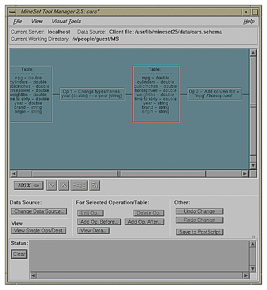
As with Edit Prev. Op, changing one operation usually affects (sometimes invalidates) subsequent operations in the history. You can select a specific operation to edit, add, or view. The View History dialog warns you when changes affect the history, shows you the new history. The row of buttons beneath the diagram window of the View History panel allows you to change the size and orientation of the diagram as detailed below.
Under the window displaying this flow chart are the zoom buttons that let you view the flow chart closer up or farther away (Figure 3-20). You can choose the zoom by using the button indicating the percentage, or by clicking the arrow buttons to increase or decrease the size. The increments of change are the same whether you use the percentage button or the arrow buttons.

This button (Figure 3-21) creates, in a separate window, an overview of the entire history chart that is synchronized with the Edit History dialog. The overview window shows you which part of the history is currently visible, and lets you pan to other parts of the history.

Next to the zoom buttons is a toggle button that lets you view the flow chart vertically or horizontally (Figure 3-22). Clicking the button switches you back and forth between the two points of view.

Under the Data Source heading is the Change Data Source... button, which lets you change the table on which the history operates. When you hold the button down, a menu appears that lets you choose
...to DBMS table
...to DBMS query
...to Data File
Selecting one of these items causes a dialog box to appear that lets you select the new data source.
| Note: As with editing the history, changing the data source can invalidate history operations. |
Under the indicator View is a View Single Ops/Dest button. When this button is pressed, the panel showing the history is hidden, and the panels showing current columns and data destinations return to view. The function of this button is the same as choosing the Single Ops and Destination option from the View pulldown menu at the top of the window.
Under the indicator For Selected Operation are three rows of buttons that become active if you click one of the operations or tables in the flow chart. Once you select an operation, you can alter it.
The Edit Op button brings up the dialog box for the selected operation, so you can make changes to it.
The Delete Op button removes the operation from the table history, and the elements that follow in the flow chart move over when it disappears.
The Add New Op. Before and Add New Op. After buttons let you insert a new operation into the table history.
The View Data button shows the data for any selected table in the history. When you click this button, a menu is displayed enabling you to select the entire dataset, or a random sample of 10, 100, or 1,000 records.
Under the indicator Other there are three buttons that affect the total history file:
The Data Destination panel (Figure 3-23) lets you direct your processed data to one of the MineSet visualization or mining tools, or to a data file.
There are three tabs at the top of this panel:
Viz Tools
Mining Tools
Data Files
These are the three possible destinations for your data. They are discussed in greater detail in later chapters dealing with the Data Destination tools.
If you choose the Viz Tool tab, the visualization tool panel appears under Data Destination (Figure 3-23).
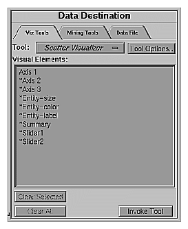
Viz Tool is a popup menu that lets you choose among Map Visualizer, Scatter Visualizer, Splat Visualizer, Tree Visualizer, Statistics Visualizer and Record Viewer, to determine the type of visual representation you want for your data.
The first five tools are described in their respective chapters.
The Record Viewer lets you view the data in the current table in a row/column spreadsheet-like tool. To use the Record Viewer select it from the tool menu, and click Invoke Tool.
Tool Options—lets you further specify options you want to set in the specified tool's configuration file.
Clear Selected—lets you undo the mapping to a selected Visual Element.
Clear All—clears all mappings.
Invoke Tool—lets you start the tool you specified (via the top button) using the configuration file named in the Saved as text field.
Each tool's requirements are listed individually in the Visual Elements pane. This pane lets you map a table column to a requirement. To do this,
Select a column by clicking its name in the Current Columns pane.
Select the requirement to which you want to map the column by clicking on that requirement in the Visual Elements pane.
The Viz Tool panel now shows the Visual Element and the column to which it has been mapped (see Figure 3-24).
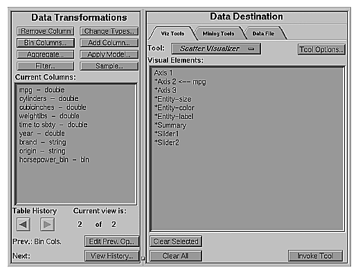
You can clear the mapping at any time by selecting the requirement that has the mapping you want to change, then clicking the Clear Selected button. You can clear all mappings using the Clear All button.
If you want to specify other details to fine-tune your mappings or to change the settings so that the data representations more clearly reflect your intentions, click the Tool Options button. A dialog box specific to each MineSet tool appears, where you can manually specify the options to use.
| Note: For details on a specific tool's options, see that tool's chapter. |
The MineSet Classifiers are described in Chapter 10, “MineSet Inducers and Classifiers,” Chapter 11, “Inducing and Visualizing the Decision Tree Classifier,” Chapter 12, “Inducing and Visualizing the Option Tree Classifier,” Chapter 13, “Inducing and Visualizing the Evidence Classifier,” Chapter 14, “Inducing and Visualizing the Decision Table,” Chapter 15, “Inducing and Visualizing the Regression Tree.” Clustering is described in Chapter 16, and Column Importance is described in Chapter 17.
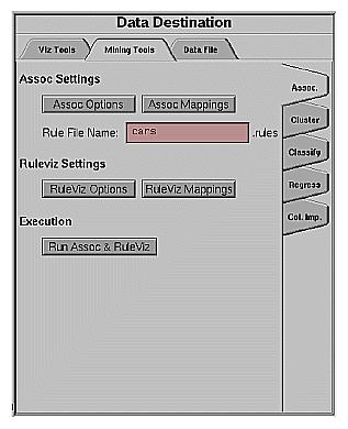
If you click the Mining Tools tab, then the Associations tab, the panel lets you take the data file you created in Data Transformations and proceed to the Rule Visualizer. Each step of the process is shown in the subpanels:
Assoc Settings—creates rule generation options and mappings from the columns in your table to elements of association rules
Ruleviz Settings—provides options to tailor the representation of the association rules in the Ruleviz tool
Execution—a button to invoke the process of finding association rules and visualizing them
If you don't want to go through this process manually, click the Execution button, and the computer will perform the process using defaults.
The Column Importance (Figure 3-26) allows you to determine how important various columns are in discriminating the different values of the label column you choose. You might, for example, want to find the best three columns for discriminating the label good credit risk so you can choose them for the Scatter Visualizer. When you select the label and click Go!, a popup window appears with the three columns that are the best three discriminators. A measure called “purity” (a number from 0 to 100) informs you how well the columns discriminate the different labels. Adding more columns can only increase the purity.
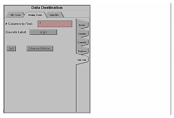
There are two modes of column importance:
Simple Mode
To invoke the simple mode, choose a discrete label from the popup menu, and specify the number of columns you want to see.
Advanced Mode
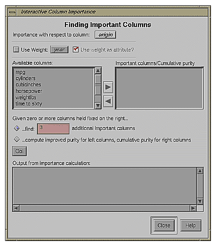
Advanced mode lets you control the choice of columns. To enter advanced mode, click Advanced Mode in the Column Importance panel. A dialog box appears, as shown in Figure 3-27. The dialog box contains two lists of column names: the left list contains available attributes, and the right list contains attributes chosen as important (by either the user or the column importance algorithm).
Advanced mode can work two different ways: finding several new important attributes, or ranking available attributes.
Finding Several Important Attributes
To enter this sub-mode, click the first of the two radio buttons at the bottom of the dialog (...find [number] additional important columns). If you click Go! with no further changes, the effect is the same as if you were in Simple Mode, finding the specified number of important columns and automatically moving them to the right column. Near each column, the cumulative purity is given (that is, the purity of all the columns up to and including the one on the line). More attributes can only increase the purity.
Alternatively, by moving columns names from the left list to the right list, you can pre-specify columns that you want included and let the system add more. For example, to select the age column and let the system find three more columns, click the age column name, then click the right arrow.
Clicking Go! lets you see the cumulative purity of each column, together with the previous ones in the list. A purity of 100 means that using the given columns, you can perfectly discriminate the different label values.
Ranking Available Attributes
Advanced Mode also lets you compute the change in purity that each column would add to all those that were already selected. For example, you might choose age, and then ask the system to compute the incremental improvement in purity that each column would yield.
To enter this sub-mode, click the second of the two radio buttons at the bottom of the dialog (...compute improved purity for left columns, cumulative purity for right columns.). This sub-mode permits fine control over the process. If two columns are ranked very closely, you might prefer one over the other (for example, cheaper to gather, more reliable, easier to understand).
Column Importance Notes
Note that with other columns, the importance of features varies from their ranking alone. For example, while net-income might be a good column individually, it might not be as important together with salary because they are likely to be highly correlated. The best set of three columns is not necessarily composed of the columns that rank highest individually. If two columns give the income in dollars and in another currency, they are ranked equally alone; however, once one of them is chosen, the other adds no discriminatory power to the set of best features.
Column selection is useful for finding the best three axes for the Scatter Visualizer, as well as for finding a good discriminatory hierarchy for the Tree Visualizer.
All floating point values (double or float) are pre-discretized using the automatic discretization. If a column has no value given to it in the left list, the algorithm did not consider it, because it either had a single value (for example, when it is discretized into one interval), or the number of records that it would separate is not statistically significant.
The Tool Manager lets you save the manipulated table for future use in a data file on the client or server. If you click the Data Files tab, the panel shown in Figure 3-28 appears.
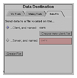
The two toggle buttons in this panel let you specify whether the file is to be saved on the server or your client machine. The selected name for the client file appears next to the Client checkbox. If you select Client, the Choose new client file button brings up a dialog for you to choose the name for the client file. If you select Server, you can type the server filename directly into the adjacent text field.
| Note: Pathnames are not permitted for server files; all server files are stored in the DataMover cache directory. |
The Tool Manager can save a description of your work to a “session file” for future use. A session file contains a description of the data source you selected, all the transformations on the data, and the mining or visualization of the data. Each session file can hold descriptions of only one data source and one data destination; thus, if you change the destination visual tool or source data table, the session file loses its links to any previous data source or destination.
Session files can be saved at any time through the entries in the File menu, described below. The name of the current session appears in the window's title bar. The Tool Manager also keeps a parallel session file, called .latest.mineset, in your home directory. It always has a record of your most recent actions in the Tool Manager. Whenever you start the Tool Manager without a session file, it reads the contents of the .latest.mineset file to return you to the state when you last ran MineSet.
Session files also can be used for running the Tool Manager in batch mode, by issuing this command at the UNIX shell prompt:
mineset_batch [-s serverPassword -d databasePassword] sessionFile |
The -s and -d options let you specify the password for logging into the server and database respectively. If you do not specify these options, mineset_batch will ask you to type in the passwords, thus these options are useful when running mineset_batch from a shell script. To specify that there is no password for either the server or database, use -s or -d followed by two double quotes, that is,
mineset_batch -s "" -d "" foo.mineset |
If you specify one of the two passwords, you must specify both.
In batch mode, the Tool Manager does not bring up tools or windows; however, it creates files for tools. For example, if the session file includes the Tree Visualizer as the data destination, running the Tool Manager in batch mode produces files for running the Tree Visualizer, but the Tool Manager does not invoke it.
At the top of the Tool Manager window (see Figure 3-1 on page 67) are four pulldown menus:
File
View
Visual Tools
Help
The following section describes each of these menus.
The File menu lets you choose what to do with your current session, which is one complete session with a tool. This includes choosing the server, data source and table, all the table manipulations, the mapping or classifying of the data, as well as opening or saving a tool history, changing the working directory, and setting preferences.
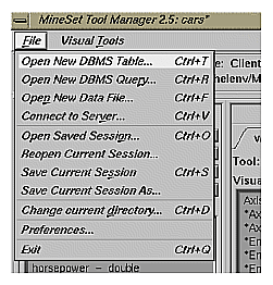
The File menu provides five sets of functions:
The first set is for selecting a data source.
Open New DBMS Table—lets you select a single table from a DBMS.
Open New DBMS Query—lets you make an SQL query against the DBMS.
Open New Data File—lets you select a table from a data file on disk.
Connect To Server—lets you open a connection to a MineSet server.
The second set is for opening or saving .mineset files.
Open Saved Session...—lets you open a .mineset file.
Reopen Current Session —lets you reopen the current session file from the disk, in case you do not want to save the current changes.
Save Current Session—lets you save a currently open .mineset file.
Save Current Session As...—lets you name (or rename) and save a currently open history as a .mineset file.
The third set is for changing the current directory.
Change Current Directory—lets you specify the directory in which the Tool Manager creates all data and visualization files.
The fourth set is for setting preferences. Here you can specify whether to
The last option, Exit, lets you end the current session and exit the Tool Manager.
The View Menu lets you select whether to see the history panel or the current columns and data destination panels.
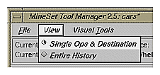
Single Ops and Destination—shows the current columns and data destination panels. This menu option performs the same function as the View Single Ops/Dest button on the history panel.
Entire History—shows the history panel. This menu option performs the same function as the View History button on the Data Transformations panel.
The Visual Tool menu lets you invoke any of the following visual tools directly:
Cluster
Decision Table
Evidence Visualizer
Map Visualizer
Rule Visualizer
Scatter Visualizer
Splat Visualizer
Statistics Visualizer
Record Viewer
Tree Visualizer
If you have created a file that runs within one of these tools, and you want to go back to it, click the tool. From within the tool, use File > Open to open the data file. These viewers are described in their respective chapters, except for Record Viewer, which is described later in this chapter, in “The Record Viewer”.
The Help menu provides information about the elements of the Tool Manager and how they work:
Click for Help—Gives help information about a particular item if you press Shift-F1, then click the item for which you want help.
Overview—Gives an overview of the online help and how to use it.
Index—Provides an index of the complete help system. This option is currently disabled.
Keys & Shortcuts—Provides the keyboard shortcuts for all of the Tree Visualizer's functions that have accelerator keys.
Product Information—Indicates what version of the Tool Manager you are using.
MineSet User's Guide—Invokes the IRIS Insight viewer with the online version of this manual.
The Tool Manager creates a .mineset file in your home directory. This is used to store the preference indicating whether to restore the most recent session on startup, as well as the default server name, login, and password. If you log in to the same server often, edit this file and specify a server name and login as follows:
default_server_name: mineset default_server_login: guest default_server_password: |
Whenever you try to log in to a server, these names appear as defaults.
 | Warning: Putting a password in a file is a great security risk. Do not place a password in the Tool Manager options file unless you want other people to know that password. |
The Record Viewer lets you view MineSet data files in a format similar to spreadsheets. There are five ways to start the Record Viewer.
Use the Tool Manager to start the Record Viewer. This invokes the Record Viewer on the data currently configured in the Tool Manager.
Double-click on the Record Viewer icon, which is in the MineSet page of the icon catalog. Since no .schema file is specified, you must select one by using File > Open.
Double-click on any MineSet .schema file. This launches the Record Viewer on that .schema file.
Drag a .schema file onto the Record Viewer icon.
Start the Record Viewer from the UNIX shell command line by entering this command at the prompt:
recordview [ file.schema ]
where file.schema is optional and specifies the name of the .schema file to use. If you do not specify a .schema file, you must use File|Open to specify one.
The Record Viewer shows the data specified by the .schema file in spreadsheet format (see Figure 3-31).
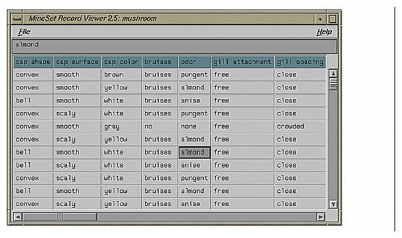
If a column is not wide enough to see a specific value, click on it to display that value at the top of the Record Viewer. You also can change the width of columns by dragging the separators between the columns.
To read a new .schema file into the Record Viewer, select File > Open. To close the Record Viewer, select File > Exit.
Note that some of the visual tools also bring up record viewers to display the current selections. These record viewers are built into the visual tools; while their behavior is the same as the Record Viewer discussed above, they do not allow opening other .schema files.
Many of the tool option dialogs have options for choosing colors. MineSet has a color list chooser that uses color swatches. This section describes how to choose, apply, and change color options for the MineSet Visualizers.
If only one color is to be chosen (for example a grid color), a single color swatch appears (Figure 3-32).
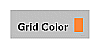
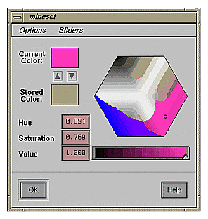
Clicking the swatch brings up a Color Browser that lets you change the color of that swatch (Figure 3-33). The Color Browser is described in more detail in the “Using the Color Browser” section, shown in Figure 3-33.
If a list of color swatches is to be chosen, the list of swatches appears (these can be empty initially), as shown in Figure 3-34.

To edit the color, click a swatch with the left mouse button. This also selects the swatch for making changes to the colors with the buttons. If you click on the swatch with the middle mouse button, the swatch is selected, but the color chooser does not appear.
Next to the list of swatches are four buttons. First is the Add button, labeled with a plus sign (+), which adds a new color at the end of the list. A swatch is added, and the color chooser appears, where you can select the color of that swatch. The Add button is disabled if the maximum number of colors is already in the list.
Next to the Add button is a Delete button, labeled with a minus sign (-). This button deletes the selected color. It is disabled if no swatch is selected, or if the list already has the minimum number of colors.
Next to the Delete button are two buttons to shift the selected color right and left. These buttons are disabled if no swatch is selected, or if the swatch is already at the end of the list.
If there are more colors in the list than room to display them, scroll arrows are added at each end of the list (Figure 3-35).

If the hardware runs out of colors, the color swatches are replaced with text labels showing the color in X notation (Figure 3-36).

The Color Browser (Figure 3-33) appears when you click a color swatch or the add button in the Colors panel of the visualizer's Configuration Options panel.
To select a color using the Color Browser:
Move your mouse cursor on top of the small circle in the colored hexagon.
Press the left mouse button, and move your mouse around the hexagon. The color beneath the small circle appears in the rectangle next to the Current Color label. This rectangle acts as your color palette while you choose a color.
Release the mouse button when the small circle is on top of a color you want. The selected swatch immediately takes on the chosen color.
You can edit several colors without dismissing the Color Browser; clicking any color in the options panel lets you edit that color in the already posted Color Browser.
Click the OK button when you decide on a color. The Color Browser window closes.