This chapter discusses the features and capabilities of the Regression Tree Inducer. Its associated visualizer, the Tree Visualizer, is described in Chapter 5. This chapter provides an overview of this tool and discusses methods of using it to generate Regression Trees. It then explains the Tree Visualizer's functionality when working with regression trees. Finally, it lists and describes the sample files provided for this tool.
 | Note: It is assumed that you have read Chapter 10, “MineSet Inducers and Classifiers,” before proceeding with this chapter. |
Regression is the task of predicting a continuous label value, given a set of descriptive attributes. A regressor is a predictive model that performs regression. Regression and classification are similar, the difference being that in classification the predicted label can take on only a small number of discrete values. For example, an iris may be classified by type as either iris-setosa, iris-versicolor, or iris-virginica. In regression, the predicted label can be any value in a continuous range, for example, an individual's annual income may be any amount greater than zero.
MineSet can build a regressor automatically from a training set using an algorithm called an inducer. The training set consists of records in the database for which the continuous label is known. For example, you could supply a database table with columns (such as age, education, occupation, hours worked per week, and so forth), and one column containing descriptive attributes (gross income). An algorithm called an inducer automatically builds a regressor from a training set.
When a regressor is generated, MineSet also generates a visualization. This visualization can help you understand the regressor and how it makes predictions. In addition, it can provide valuable insight into the data itself. Once generated, a regressor can be used to predict the label value for unlabeled records.
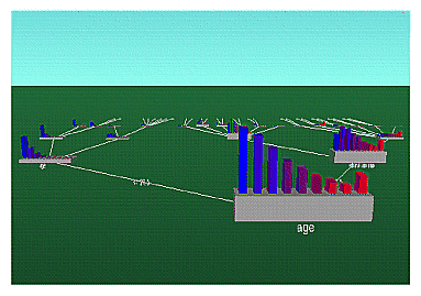
The underlying structure used for regression is a Regression Tree, such as the one shown in Figure 15-1.
There are two ways to run the Regression Tree Inducer:
From the Tool Manager.
Connect to the server and select a data source (see “Choosing a Data Source” in Chapter 3).
From the File menu, choose Open New Data File. Log in to a server, and enter the filename. For the example shown here, the filename entered would be /usr/lib/MineSet/data/adult.schema. In the Continuous Label popup menu of the Data Destination pane you see a list of continuous attributes. Of the several continuous attributes available, one is automatically selected as the label option. You may change this. Regression Tree Inducer is automatically shown as the inducer. To run the Inducer, click Go!.
The status window shows the progress and statistics, and the Tree Visualizer is launched automatically.
From the command line.
To induce a Regression Tree classifier from the command line, refer to Appendix I, “Command-Line Interface to MIndUtil: Analytical Data Mining Algorithms.”
To access the options for configuring the Regression Tree Inducer, select the Mining Tools tab on the Data Destination panel (Figure 15-2). From the tabs at the right, select Regress. The selected inducer is the Regression Tree, the only regression model currently available in MineSet. Your selections in the Mode menu determines the options available in the Further Inducer Options menu. After you have made your selections in these menus, click Go! to induce the regressor.
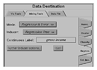
The Continuous Label menu provides a list of possible continuous labels. This list includes all attributes that take on numeric values. Select the label attribute you wish to model. For instance, to generate a regressor for predicting gross income, select “gross income”. (See “Training Set” in Chapter 10). If there are no continuous attributes, the menu shows No Continuous Label, and the Go! button is disabled. Regressors can only be generated for continuous attributes. If the dataset does not contain a continuous attribute you may add a new continuous column using the Tool Manager's Data Transformations panel.
The generated regressor is named with the prefix of the session filename (as determined in Tool Manager) and the suffix -rt.regress. By default, all regressors are stored on the server in the file_cache directory, which defaults to mineset_files.
These regressors can be used to predict the labels for unlabeled datasets. To apply a stored regressor, you need to select a dataset of records with the attributes used by the regressor. The regressor will predict a new continuous label value for each record. See “Applying a Model” and “Backfitting in Error Estimation” in Chapter 10.
Selecting Further Inducer Options displays the Inducer Options dialog box (Figure 15-3). to appear. This dialog box consists of four panels:
The top panel indicates the choices you made in the Tool Manager's Data Destination panel.
The second panel from the top lets you set the weight attribute. See “Weight Setting” in Chapter 10.
The bottom-left panel lets you specify other Inducer Options.
The bottom-right panel lets you specify the Error Estimation Options (unless the mode you chose in the Data Destination panel was Classifier Only, in which case this area is empty). The options shown in this panel depend on the type of Error Estimation you chose (see “Error Options for Inducers” in Chapter 10).

To fine-tune the Regression Tree induction algorithm, you can change the following Regression Tree Inducer options (see Figure 15-3).
-
By default, there is no limit to the height (number of levels) in the Regression Tree. You can limit the height by clicking the check box and typing a number for the limit. Limiting the number of levels speeds up the induction and is useful for studying the Regression Tree without the distraction of too many nodes. Note that restricting the size decreases the run time, but may increase the error rate. Setting this option does not affect the attributes chosen at levels before the maximum level.
-
This option allows you to specify which criterion will be used to select among competing attribute splits during tree induction. For regression trees, MineSet supports four splitting criteria:
Variance chooses splits that minimize the within-node variance at each point in the tree. When generating a leaf, the prediction at the leaf is the mean of the label values of the records reaching that leaf. Variance is the squared difference between each of the values in the set, divided by the total number of elements or values. This mode is most commonly used statistically.
Absolute Deviation chooses splits that minimize the absolute deviation within the node at each point in the tree. When generating a leaf, the prediction at the leaf is the median of the label values of the records reaching that leaf.
Normalized Variance (the default) is variance divided by the log (base 2) of the number of child nodes.
Normalized Absolute Deviation is absolute deviation divided by the log (base 2) of the number of child nodes.
For a given problem, it is difficult to know which criterion will be best. Try each, and select the one that leads to the lowest error estimate, or the Regression Tree you find easiest to understand.
-
This is a lower bound on the weight (or the number of records if weight was not set) that must be present in at least two of the node's children. The default for this option is 5. For example, if there is a three-way split in the node, at least two out of the three children must have a weight of five or more. This provides another method of limiting the size of the Regression Tree.
Increasing the split lower bound tends to increase the reliability of the probability estimates, because the number of records at each leaf is larger. It also creates smaller trees and decreases the induction time. If you expect the data to contain noise (errors or anomalies), increase the split lower bound. If your dataset is very small (< 100 records), you might want to decrease the split lower bound.
-
Cost complexity pruning attempts to generate optimally sized trees by trading off the error rate of the tree (its cost) and the number of leaves in the tree (its complexity). During cost complexity pruning the training set is partitioned into a learning set and a pruning set. The learning set is used to grow a pruning tree. This tree is pruned to generate a sequence of trees with decreasing complexity. The pruning set is then used to identify the minimum cost tree in this sequence. The size of the minimum cost tree is noted. The learning and pruning sets are recombined and used to grow a tree. This tree is then pruned to the size of the minimum cost tree.
The cost complexity pruning parameter allows you to select trees smaller than the minimum cost tree. The parameter indicates the number of standard errors more costly than the minimum cost tree that you are willing to accept. Setting the parameter to zero selects the minimum cost tree; setting the parameter to 0.5 selects the minimum size tree that had an error rate no more than 0.5 standard errors worse than the minimum cost tree. The default setting, 1, selects the minimum size tree that has an error rate no more than one standard error worse than the minimum cost tree. Higher numbers indicate more pruning. If your data may contain noise (errors and anomalies), increase the number to create smaller trees. If the tree is pruned back to a single node, decrease the number to decrease the amount of pruning and show more of the trees structure.
Pruning is slower than limiting the tree height or increasing the split lower bound because a full tree is built and then pruned. Pruning, however, is done selectively, resulting in a more accurate regressor.
When evaluating a classifier the natural metric is error (the number of examples for which the classifier predicts the wrong label). When a loss matrix is supplied, different types of misclassification errors may have different associated costs. In this situation loss is a natural measure.
For regression, where the task is to predict a real value there is no single natural evaluation metric. The two measures that are frequently used are mean squared error and mean absolute error. In Mean Squared Error, the mean of the squared difference between the predicted label value and the actual label value is used. In mean absolute error, the mean of the absolute value of the difference between the predicted label value and the actual label value is used.
A Regression Tree visualization is similar to Decision Tree visualization. Like a Decision Tree, a Regression Tree consists of nodes connected by lines (see Figure 15-1).
There are two types of nodes: decision nodes and leaf nodes.
Decision nodes specify the attribute that is tested at the node. Values (or ranges of values) against which the attributes are tested are shown at the lines. Each possible value for the attribute matches exactly one line. For example, the root of the Regression Tree in Figure 15-1 tests the attribute age; the two lines emanating from the node partition values for that attribute (< 27.5, => 27.5) so that every possible value matches either the right branch or the left branch. If the value is unknown and there is no line labeled with a question mark, the mean or median label values at the current node is predicted.
Leaf nodes in a Regression Tree predict a value. Follow the left-most branch in Figure 15-1 from the root to the leaf labeled 5540.038. Note that the Regression Tree predicts that people under 23.5 who work less than 35.5 hours per week will average a gross income of $5540.40.
The bars atop nodes in a Regression Tree are different than the bars atop nodes in a Decision Tree. In a Decision Tree each bar corresponds to a specific discrete label value. In a Regression Tree each bar corresponds to a subrange of continuous label values. In a Decision Tree the bars have a simple mapping throughout the entire tree. For example, in Figure 11-1 of Chapter 11, “Inducing and Visualizing the Decision Tree Classifier,” the leftmost bar of each node indicates the weight (number) of records with the iris-setosa label. By contrast, in a Regression Tree the range of continuous label values covered by each node can be different. The bars at each node form a histogram indicating how the weight (number) of records is distributed over this range. The leftmost bar always shows the weight (number) of records with the lowest label values. But the size of that subrange and its midpoint maybe different at every node. In a Decision Tree, the color of a bar indicates the discrete class label. In a Regression Tree, the color of a bar indicates the midpoint of the subrange that bar covers.
In the Decision Tree, each bar corresponds to a label value. The height of the bar indicates the total weight of records with that label value at that node. The bars are consistent throughout the entire tree. For example, if you run the Regression Tree on the iris dataset the leftmost bar at the root node indicates the weight (number) of records with the iris-setosa label. The left most bar at each node indicates the weight (number) of records with the label iris-setosa.
In a Regression Tree, the set of bars on a node collectively form a histogram of the label values at that node. The number of bars is determined by the weight of records at the root. The color of the bars indicates of the range. The maximum range is indicated by blue on the left and red on the right. A node which only covers records with a limited range of label values will have a histogram that doesn't range from blue to red.
The base of each node has a height. The height corresponds to the weight of the training set records that have reached this node (this is the number of records if weight was not set). In general, the higher the weight, the more reliable the distribution at a node.
Pointing to a node causes the following information to be displayed:
Subtree weight—The weight of the training set records in the subtree below the node pointed to. This value is mapped to the height of the base.
Mean: the mean of the continuous label
Standard deviation: the standard deviation of the continuous label. The higher the standard deviation, the less reliable the model.
Median: the median of continuous label.
Absolute deviation: absolute deviation of the continuous label. The higher the absolute deviation, the less reliable the model.
All possible outcomes are marked on the horizontal lines emanating from each decision node. Each line indicates the value (or range of values) against which the attribute of that node was tested.
To predict a value for a record, start at the root, and test how to branch at every decision node. By following the appropriate lines based on the record's attribute values, you reach a leaf node. The label, or prediction, associated with the leaf node is the predicted value of the record.
The external controls for the visualizer associated with a Regression Tree are the same as those for the Tree Visualizer. For a description of these controls, see “External Controls” in Chapter 5.
One particularly useful control for regression trees is to select a node, and from the menu Selections select the menu item Normalize Sub Tree (or press Ctrl-N). This will normalize the height and color range of the tree using the current node. By default the tree is normalized to the root node.
Another useful control is to click the right mouse button when pointing to a node. This shows the list of children of that node.
The pulldown menus for the visualizer associated with a Regression Tree are the same as those for the Tree Visualizer. For a description of these menus, see “Pulldown Menus” in Chapter 5, and “The Search and Filter Panels” in Chapter 11.
The following examples show cases in which regression might be useful and highlight some of the capabilities of the Regression Tree Inducer. Each of these examples is associated with a sample data file provided with MineSet. By running the inducer, you can generate the -rt.regress files described below.
| Note: The data files, which have a .schema extension, are located in /usr/lib/MineSet/data on the client workstation; and the regressor visualization files, with a -rt.treeviz extension, reside on the client workstation in /usr/lib/MineSet/treeviz/examples. |
The churn dataset contains generated information on the calling patterns of a telecommunication company's customers. In the classification examples, this dataset is used to determine which factors lead a customer to churn, or leave the company for one of its competitors. In this regression example, we will try to determine what factors influence how much the company charges each customer per day.
The file churn-rt.treeviz shows the Regression Tree generated on this data set to predict the total day charge. Interestingly, the tree branches on only one attribute throughout, total day minutes, continuously dividing this attribute further and further into progressively smaller ranges. This is because the relationship between total day minutes and total day charge is completely deterministic—the customers are charged only for the minutes they use the system. The Regression Tree is quickly able to locate and capitalize on this fact.
The cars dataset contains information about different models of cars from the 1970s and the early 1980s. Attributes in this data set include weight, acceleration and miles per gallon. The file cars-rt.treeviz shows the Regression Tree regressor induced on this data set, using miles per gallon as the continuous label.
By clicking on the top node, we see that the average mpg of cars in this dataset is around 23.5. The first split in the Regression Tree for this dataset shows that the most important factor contributing to the mileage of a car is its weight. The Regression Tree has discovered that heavier cars get lower mileage, a fact that may be obvious to a human observer, but is insightful for an automated discovery program. By looking at the two children of the base node, we note that the right child is bluer than the left one, that is it gets fewer miles per gallon. By highlighting the nodes, we see that cars that weigh less than 3018 lbs. get around 28.3 mpg, while cars weighing more get around 16.6 mpg.
Heading over to the heavier cars, we see that the next split is on the horsepower of the car, and that more powerful cars tend to get lower mileage. The split at the next level that is on the year the car was made, with newer cars getting better mileage. Now, let's look for an unusual car. Using the filter panel, let's try and find a node with a mean mpg < 24 but with a maximum > 30. Doing this filter, we quickly reduce the tree to one node, cars weighing less than 3018 lbs, with more than 77 horsepower, and made before 1980. In this category, there is an unusual car; by selecting the rightmost bar on that node and sending this information to the Tool Manager via the Selections > Show Original Data menu item, we see that this car is a 1978 Dodge, weighing around 2000 lbs, with 83 hp, but getting a high 33.5 miles per gallon.
The adult dataset contains information about working adults, extracted from the U.S. Census Bureau. It contains data about people older than 16, with a gross income of more than $100 per year, who work at least one hour a week. We can use the Regression Tree Inducer to determine which factors influence a person's salary; as well as to give a rough prediction of what that person's salary would be, given the other information.
The file adult-rt.treeviz shows the Regression Tree regressor induced on the adult dataset, using gross income as the continuous label. Note that this data set is large (around 50000 records), and therefore inducing the regressor on this data set may take a few minutes on your workstation.
The bars at the top node provide a histogram of salary values in the Census Bureau's data. Note that the amount of data available decreases as the salary level increases. We have a lot of data for people earning around $3,000 a year, but less so as that figure increases. This trend is reversed in the last part of the histogram that indicates a sizeable amount of data on people earning roughly $100,000 per year. This discrepancy might be the result of either a genuine trend in the data, or a biased sampling.
The first division in the Regression Tree is on the age attribute. As expected, younger people generally make less money than older people. Brushing the top node and its two children nodes, we can see some summary statistics for these three groupings of people. We note that the mean salary for everyone in this study is around $33,500, while the mean salary of people under 27 is around $14,300; and the mean salary of those over 27 is around $40,000.
Following the next two divisions of people under 27, we see that the tree again splits them into two categories: those 23 and under, and those over 23. Interestingly, the split past these two divisions is the same, and on the hours per week attribute, indicating that for both age ranges the more hours worked, the higher one's gross income.
Now, focusing on those over 27, we find that the tree splits immediately on the amount of education a person has had. Those with an education number 13 and over (which corresponds to a bachelor's degree), tend to make more money. By looking over the two children of the education number split, we can see that most of the people making around $90,000 a year have at least some advanced education.
We can use the filter panel, to quickly locate those categories of people making on average over $50,000 a year. In the filter panel, select mean > 50000. Top level nodes disappear in this filter, as making that amount of money is a rare occurrence. People with a bachelor's degree who are over 27 fall in this category. By following the left branch of the first split to the end, we find another group of people in this category: married men over 36 years old, who work over 35 hours a week and have a good education (10 years or more).
If we revisit the filter, and look for nodes with an absolute deviation of larger than $25,000, we can find those people whose economic condition offers the widest variability. The first remaining node in this filter is those people over 27 and with a bachelor's degree. The histogram above this node shows a distribution centered around its mean, but with an unusual number of people making around $100,000 a year.
Each record in this dataset describes five characteristics of iris flowers, petal width, petal length, sepal width, sepal length, and iris type. Our goal in this regression is to predict the petal width based on the other characteristics. The file iris-rt.treeviz shows the results of the Regression Tree Inducer run on this dataset in order to predict petal width.
Looking at the top node, we see a gap in the petal width values, where no flowers exist. The Regression Tree Inducer splits on this data set first using the petal length variable. If the petal length is less than 2.6, only a restricted set of petal widths seems possible. On the other hand, petal length values greater than 2.6 indicate a more even distribution with larger corresponding petal lengths. The mean petal width for those irises with petal lengths less than 2.6 is 0.24, while the corresponding mean petal width for those with lengths greater than 2.6 is 1.68. Following the large petal length irises, we see that the tree splits again on petal length, this time on the value 4.85. These two consecutive splits on the same variable point to some kind of restricted functional relationship between these two variables.
Going back to those irises with a petal width less than 2.6, we see that the following split is on the sepal width attribute. Interestingly, the values in this part of the tree seem segregated, with those irises with sepal width less than 3.25 taking on values in three narrow but separated ranges.
This dataset is a diabetes diagnosis problem using statistics gathered from an Indian tribe in Phoenix, Arizona. The file pima-rt.treeviz shows the results of running the Regression Tree Inducer on this dataset, using the plasma glucose level as the predicted continues variable.
The first split in this tree is on the diabetes indicator, showing that people with diabetes tend to have a higher plasma glucose level than those without (141 versus 110). The next split is the 2-hour serum insulin attribute, where values greater than 125 lead to higher plasma glucose.
The Regression Tree predicts by following the decisions at each of the nodes from the top node, while examining new records. For example a diabetic patient with 2-hour serum insulin of 110 would have a predicted plasma glucose level of 105.