This chapter discusses the features and capabilities of the Decision Tree Inducer. Its associated visualizer, the Tree Visualizer, is described in Chapter 5. This chapter provides an overview of this tool and discusses the ways of using it to generate Decision Tree classifiers. It then explains the Tree Visualizer's functionality when working with the main window. Finally, it lists and describes the sample files provided for this tool.
 | Note: It is assumed that you have read Chapter 10, “MineSet Inducers and Classifiers,” before proceeding with this chapter. |
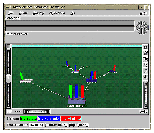
A Decision Tree classifier assigns each record to a class. The underlying structure used for classification is a Decision Tree, such as the one shown in Figure 11-1.
A Decision Tree classifier is induced (generated) automatically from data. The data, which is made up of records and a label associated with each record, is called the training set (see Chapter 10, “MineSet Inducers and Classifiers”).
The Decision Tree Inducer requires a training set, as described in the “Training Set” in Chapter 10. Files are generated by extracting data from a source (such as a MineSet ASCII or binary file, or a table in an Oracle, INFORMIX, or Sybase database). To apply the generated classifier, you should have a dataset of records with the attributes used by the classifier, except that the label need not be present.
There are two ways to run the Decision Tree inducer:
From the Tool Manager.
Connect to the server and select a data source (see “Choosing a Data Source” in Chapter 3).
From the File menu, choose Open New Data File. Log in to a server, and enter the filename. For the example shown here, the filename entered would be /usr/lib/MineSet/data/iris.schema as the filename. You'll see four continuous attributes and one discrete attribute in the Data Transformation panel. Since there is only one discrete attribute, the label option automatically shows it. Select the Decision Tree inducer, and ensure you have selected the Classifier & Error mode. To run the Inducer, click Go!.
The status window will show the progress, statistics, and the Tree Visualizer will be launched automatically.
From the command line.
To induce a Decision Tree classifier from the command line, refer to Appendix I, “Command-Line Interface to MIndUtil: Analytical Data Mining Algorithms.”
To access the options for configuring the Decision Tree inducer, select the Mining Tools tab on the Data Destination panel (Figure 11-2). From the tabs at the right, select Classify. Ensure that the inducer you select is Decision Tree (the default). Your selections in the Mode and Inducer menus determine the options available in the Further Inducer Options menu. After you have made your selections in these menus, click Go! to run the inducer, which, in turn, creates the classifier.
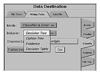
The Discrete Labels menu provides a list of possible discrete labels. Discrete attributes (binned values, character string values, or a few integers) have a limited number of values. You should select a label attribute with few values; for instance, two or three (see “Training Set” in Chapter 10). If there are no discrete attributes, the menu shows No Discrete Label, and the Go! button is disabled. You then must create a discrete attribute by binning or adding a new column using the Tool Manager's Data Transformations panel.
The generated classifier is named with the prefix of the session filename (as determined in Tool Manager) and the suffix -dt.class. By default, all classifiers are stored on the server in the file_cache directory, which defaults to mineset_files. These classifiers can be used for future classification of unlabeled records; that is, they can be used to predict the labels for unlabeled datasets (see “Applying a Model” and “Backfitting in Error Estimation” in Chapter 10).
If you have installed the multiprocessor version of MineSet, it is possible to compute tree-based algorithms in parallel whenever a branch contains over 1000 records. Each node on the tree estimates the best possible split on the corresponding level, and these tasks are performed in parallel. The maximum number of threads a program can spawn is determined automatically by default. You can control the number of threads by changing the parallelization mode in the Preferences panel of Tool Manager (see“The File Menu” in Chapter 3). Parallelization may cause memory fragmentation, causing the largest data sets that can be computed in parallel to be smaller than the largest data sets that can be computed on a uniprocessor.
Selecting Further Classifier Options causes the Classifier Options dialog box (Figure 11-3) to appear. This dialog box consists of four panels:
The top panel indicates the choices you made in the Tool Manager's Data Destination panel.
The second pane from the top lets you set the loss matrix and the weight attribute. See “Loss Matrices” and “Weight Setting” in Chapter 10.
The bottom-left panel lets you specify further Inducer Options.
The bottom-right panel lets you specify the Error Estimation Options (unless the mode you chose in the Data Destination panel was Classifier Only, in which case this area is empty). The options shown in this panel depend on the type of Error Estimation you chose (see “Applying Models, Testing Models, and Fitting New Data” in Chapter 10).
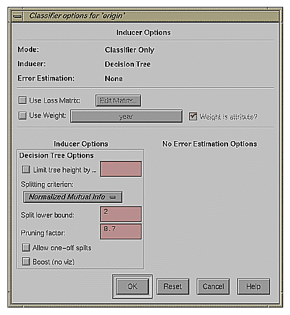
To fine-tune the Decision Tree induction algorithm, you can change the following Decision Tree inducer options (see Figure 11-3).
-
By default, there is no limit to the height (number of levels) in the Decision Tree. Limit the height by clicking the checkbox and typing a number for the limit. Limiting the number of levels speeds up the induction and is useful for studying the Decision Tree without the distraction of too many nodes. Note that restricting the size decreases the run time but might increase the error rate. Setting this option does not affect the attributes chosen at levels before the maximum level.
-
This option offers three splitting criteria selections. The definitions below are technical. For a given problem, it is difficult to know which criteria will be best. Try them all, and select the one that leads to the lowest error estimate - or to a Decision Tree you find easiest to understand.
Mutual Info is the change in purity (that is, the entropy) between the parent node and the weighted average of the purities of the child nodes. The weighted average is based on the number of records at each child node.
Normalized Mutual Info (the default) is the Mutual Info divided by the log (base 2) of the number of child nodes.
Gain Ratio is the Mutual Info divided by the entropy of the split while ignoring the label values.
Normalized Mutual Info and Gain Ratio give preference to attributes with few values.
-
This is a lower bound on the weight (normally the number of records if weight was not set) that must be present in at least two of the node's children. The default for this option is 2. For example, if there is a three-way split in the node, at least two out of the three children must have a weight of two or more (two records or more if weight is not set). This provides another method of limiting the size of the Decision Tree.
Increasing the split lower bound tends to increase the reliability of the probability estimates, because the number of records at each leaf is larger. It also creates smaller trees and decreases the induction time. If you expect the data to contain noise (errors or anomalies), or if you use the tree for estimating probabilities (see “Applying a Model” in Chapter 10), increase the split lower bound to 5 or more. If your dataset is very small (< 100 records), you might want to decrease this number to 1.
-
A Decision Tree is built based on the limits imposed by Limit Tree Height and Split Lower Bound. Statistical tests are then made to determine when some subtrees are not significantly better than a single leaf node in which case those subtrees are pruned.
The default pruning factor of 0.7 indicates the recommended amount of pruning to be applied to the Decision Tree. Higher numbers indicate more pruning; lower numbers indicate less pruning. If your data might contain noise (errors or anomalies), increase this number to create smaller trees. The lowest possible value is 0 (no pruning); there is no upper limit.
Pruning is slower than limiting the tree height or increasing the split lower bound because a full tree is built and then pruned. Pruning, however, is done selectively, resulting in a more accurate classifier
Boosting
Boosting is employed to improve accuracy of classification, although it is a time-intensive process. Visualization is not performed during boosting.
The estimated error appears in the status window, as the process runs. This estimated error is the result of the algorithm repeatedly assigning new weight distributions to the training set, and inducing a classifier on the reweighted sets. Estimating error in this manner is normally done after you have done a visualization to gain insight into the dataset. See “Boosting: Accuracy is Sometimes Crucial” in Chapter 10 for more information on boosting.
Allow one-off splits
Clicking this checkbox allows the inducer to make two-way splits on nominal attributes that have more than two values. Normally, splits on nominal attributes have as many lines as they have values (see the section on Decision Nodes, below). For example, a split on the attribute “color” might have lines for red, green, yellow, and blue. If one-off splits are enabled, then the inducer can also make splits with just two lines, for example red, and not red. One-off splits isolate exactly one of the possible values that the column can have. These kinds of splits may be useful when the data contains attributes with many possible values, some of which are exceptionally good at discriminating the label.
The Tree Visualizer's main window shows the Decision Tree. This Decision Tree consists of nodes connected by lines (see Figure 11-1).
decision
leaf
Decision nodes specify the attribute that is tested at the node. Values (or ranges of values) against which the attributes are tested are shown at the lines. Each possible value for the attribute matches exactly one line. For example, the root of the Decision Tree in Figure 11-1 tests the attribute petal_length; the two lines emanating from the node specify the ranges of values for that attribute (< = 2.6 and >2.6,) so that every possible value matches either the right branch or the left branch. If the value is unknown and there is no line labeled with a question mark (?), the majority class of the current node is predicted.
Leaf nodes in a Decision Tree specify a class. Follow the left branch in Figure 11-1 from the root to a leaf labeled iris-setosa. Note that the Decision Tree classifier classifies all records with petal_length < = 2.6 inches as belonging to the class iris-setosa.
The vertical bars atop each node show the distribution of the classes at the node. The base of each node has a height and a color. The height corresponds to the weight of the training set records that have reached this node (this is the number of records if weight was not set). In general, the higher the weight, the more reliable the class distribution at every node.
The color of the base indicates the error estimate of the subtree: indigo shows high error, grey indicates medium, white indicates low error. The color of the base is black if no test set records reached a node; thus, there is no error estimate.
Pointing to a node causes the following information to be displayed:
Subtree weight — The weight of the training set records in the subtree below the node pointed to. This value is mapped to the height of the base.
Test set error/loss — An estimate of the subtree error (or loss if a loss matrix was given). The number after the +/- is the standard deviation of the estimate. The higher the standard deviation, the less accurate the error estimate. The error/loss estimate and the standard deviation are less reliable for leaves with few records or when the test set error is close to 0% or 100%.
Test set weight — The weight of records from the test set that reached the node (number of records if weight was not set).
Purity — A number from 0 to 100 indicating the skewness of the label value distribution at the node. If a node has records from a single class, the purity is 100. If the label values have the same weight, the purity is 0. The purity is computed after backfitting.
When backfitting is enabled and Display training set as disks checked on, the vertical bars show the distribution of the training set as disks. The heights of the disks are on the same scale as the heights of the bars. You should expect the disks to appear about as high on the bars as the value used for the Holdout ratio in Further inducer options.
Note that only Classify & Error yields the test set error/loss and weight. You can use the Test Classifier option (see “Applying Models, Testing Models, and Fitting New Data” in Chapter 10) to generate a visualization based on an existing classifier and a test set.
All possible outcomes are marked on the horizontal lines emanating from each decision node. Each line indicates the value (or range of values) against which the attribute of that node was tested.
To classify a record, start at the root, and test how to branch at every decision node. By following the appropriate lines based on the record's attribute values, you reach a leaf node. The label, or class, associated with the leaf node is the predicted classification of the record.
Some decisions are quickly made and take a shorter path (for example, petal_length <=2.6 implies iris-setosa). Other decisions can take a longer path (for example, the right branches, petal_length > 2.6 and petal_width > 1.65). In general, every leaf corresponds to a rule that is the conjunction of all tests at the decision nodes and all the values (or ranges of values) on the lines leading to it from the root.
In the root of the tree shown in Figure 11-1, the error rate is 6%, with a standard deviation of 3.39%. The standard deviation is high because the file is small, and the test set only has 50 records. The purity is 0.0, indicating that the distribution is uniform.
The left child of the root has 0 test set error and a purity of 100 because all records with petal_length <=2.6 inches are of the iris-setosa class; thus, the prediction of iris-setosa is likely to be very accurate for all records with petal_length <=2.6 inches. The right child of the root has an estimated error of 8.57%. In this child, which matches records whose petal_length > 2.6 inches, there are no records belonging to the iris-setosa class; thus, the class is more likely to be iris-versicolor or iris-virginica. Because only two possibilities exist at this node, there is a higher purity than at the root (36.91).
The Decision Tree leaves segment the data into clusters sharing the same classification rule (path that leads to each leaf). By looking at the leaves, it is possible to see clusters that share the same set of properties.
The external controls for the visualizer associated with the Decision Tree classifier are the same as those for the Tree Visualizer. For a description of these controls, see “External Controls” in Chapter 5.
One particularly useful control for decision trees is to click the right mouse button when pointing to a node. This shows the list of children of that node.
The pulldown menus for the visualizer associated with the Decision Tree classifier are the same as those for the Tree Visualizer. For a description of these menus, see “External Controls” in Chapter 5.
Select Search Panel and Filter Panel in the Show menu to bring up a dialog box that lets you specify criteria to search/filter for objects (Figure 11-4). The panels are the same ones described in “The Search Panel” in Chapter 5; however, the item choices for decision trees are always the same. These are described below.

The search/filter can be restricted to specific class labels, either by selecting the values in the class list or by using the class item, which allows more powerful comparison operators (such as Matches). Other items are described below:
Subtree weight lets you restrict the search/filter to bars or bases (depending on the choice of the radio button bars/bases) with a given weight (number of records if weight is not set) for the subtree. For example, you can restrict the search to bars containing a weight of at least 50.
Test attribute lets you restrict the search/filter to nodes labeled by the given value that the node is testing. Note that decision node labels represent the test attribute, while leaf node labels show the predicted label. For example, if you select Test attribute contains age, only nodes that test the value of age are considered.
Test value lets you restrict the search/filter to nodes having an incoming line labeled with a value you specify.
Percent lets you restrict the search/filter to bars representing a percentage of the overall weight at a node. For example, you might want to find all nodes such that a given class accounts for more than 80 percent of the weight. To do this, click the class label, and select Percent > 80. Setting this item is meaningless if you select bases and not bars (the value for the bases is 0).
Purity lets you restrict the search/filter to nodes with a range of purity levels. For example, if you want to look at pure nodes (with one class predominant), you can select Purity > 90.
Test-set subtree weight lets you restrict the search/filter to subtrees with a given test-set weight (number of test-set records if weight is not set).
Test set error/loss lets you restrict the search/filter to nodes with a range of estimated error/loss.
Mean error/loss standard deviation lets you restrict the search/filter to nodes with a range of estimated standard deviation for the test set error/loss.
Level lets you restrict the search/filter to a specific level or range of levels. For example, you can search only the first five levels.
The following items and options are less useful for decision trees.
Once the search is complete, yellow spotlights highlight objects matching the search criteria. To display information about an object under a yellow spotlight, move the pointer over that spotlight; the information appears in the upper left corner, under the label “Pointer is over:.” To select and zoom to an object under a yellow spotlight, left-click the spotlight; if you press the Shift key while clicking, zooming does not occur.
Once the filtering is complete, the scene shows only nodes matching the filtering criteria.
The following examples illustrate cases in which the Decision Tree inducer can be useful. Each of these examples is associated with a sample data file provided with MineSet. By running the inducer, you can generate the -dt.treeviz files described below.
| Note: The data files, which have a .schema extension, are located in /usr/lib/MineSet/data on the client workstation. The classifier visualization files, which have a -dt.treeviz extension, reside on the client workstation in /usr/lib/MineSet/treeviz/examples. |
When customers change their phone carrier from one telecommunications company to another, this is termed “churning.” This is a common problem in the telecommunications industry. The file /usr/lib/MineSet/treeviz/examples/churn-dt.treeviz shows a Decision Tree classifier induced for this problem. The file was generated by running the inducer on /usr/lib/MineSet/data/churn.schema with the label set to churn (yes, no). The file given is fictitious, but based on patterns found in real data.
Note that in this tree the root split is on the amount of time the customers talk during the day (total day minutes). Customers who talk more than 264 minutes per day churn at a significantly higher rate than those who don't (60% versus 11%). These also are probably the most profitable customers.
The left subtree represents customers who talk less than 264 minutes per day. They have a churn rate of 11%; but if they make more than three customer service calls, the churn rate increases to 49%.
The right subtree represents customers who talk over 264 minutes per day. They have a churn rate of 59%; but if they have a voice-mail plan, the rate decreases to 9.3%. If they do not have a voice-mail plan, the churn rate is almost 75%.
The cars dataset contains information about different models of cars from the 1970s and early 1980s. Attributes include weight, acceleration, and miles per gallon (mpg). The file /usr/lib/MineSet/treeviz/examples/cars-dt.treeviz shows the Decision Tree classifier induced for this problem. This file was generated by running the inducer on /usr/lib/MineSet/data/cars.schema with the label set to origin (Japan, U.S., Europe). If you have a dataset of car attributes, you might want to know what characterizes cars of different origins.
Note that in the tree the left split is on brand. The root split is not brand because the Decision Tree inducer penalizes multi-way splits; and the split on cubic_inches was deemed a better discriminator. You can use the Tool Manager Remove Column transformation to hide the brand, thus making the problem more interesting.
In the Decision Tree, you can see that cubic inches is an excellent discriminator for U.S.-made cars. Cars with large engines (>169.5 cubic inches) are all made in the U.S., but smaller cars are made everywhere. By choosing Selections > Show Original Data, you can see that the one car with a big engine that was not made in the US is a Mercedes. Note that in this tree, the root node (that is, the entire training dataset) has many more U.S. cars (62.50%), yet after a single split on the cubic inches attribute, it is more difficult to predict the origin of cars with small engines. The purity of the root is 16.2 showing that there is one class (U.S., in this case) that is dominant. The right node (cubic inches > 169.5) has purity 96.81, indicating that we have identified a very pure subpopulation (almost all cars with large engines were made in the U.S.). Indeed, the error rate for the right subtree is estimated at 0% (green base). The left node from the root has purity 0.23 and a much higher error rate of 31.25% (orange base). This subproblem is much harder than the original one: the number of records for each class is approximately the same.
The adult dataset contains information about working adults. This dataset was extracted from the U.S. Census Bureau. It contains data about people older than 16, with a gross income of more than $100 per year who work at least one hour a week. You might want to know how to characterize males and females. The file /usr/lib/MineSet/treeviz/examples/adult-sex-dt.treeviz shows the Decision Tree classifier induced for this problem. This file was generated by running the inducer on /usr/lib/MineSet/data/adult.schema, with the label set to sex. Note that this dataset contains almost 50,000 records; thus, running the Decision Tree Inducer can take several minutes when you run this on your workstation.
The resulting visualization provides the following insights:
Relationship is a giveaway attributes for some values. Husbands usually are male. (Interestingly, there is one husband that is a female, showing data quality problems at the Census Bureau, which does not recognize same-sex marriages.) Similarly, if the person is a wife, the person is usually a female, except for three records that show otherwise.
To make the problem more interesting, remove the relationship attribute and generate a new Decision Tree. Note that
The most important attribute is marital status.
From the height of the bases, most people are either divorced, married to a civilian spouse, or never married. Few are married with spouse absent, separated, married to armed-forces spouse, or widowed.
The distribution at the root shows more males in this dataset. (This database contains information about working adults and is not representative of the entire population.)
The left-most node contains divorced working adults. We can see that the distribution is more balanced than at the root (60% female, 40% male). The second node contains married working adults. We can see that 89% are males. The third node contains working adults that have never married. Their numbers are approximately equal to those in the divorced group, with slightly more males. The right-most node contains working widowed adults, of which 81% are females (probably because of their higher life expectancy).
If you want to target working females for a new product, you can use the search panel to identify segments that have a large population of females. You can do this by choosing
sex matches female (click female on the top portion of the window).
subtree weight > 1000
percent > 80
Three yellow spotlights show the matching nodes. Since two are on one path, look at the node closest to the root (on the right). The paths translate into the rules
marital status = Widowed implies that 81.23% are female marital status = Divorced and occupation = administrative clerical implies that 87.67% are female |
In this training set, 1233 (widowed) and 1045 (divorced and occupation) females satisfy these rules out of 16,192 at the root. This simple segment contains over 14% of working women.
If you have a dataset of working adults, you might want to find out what factors affect salary. You might then divide the records into two classes: those adults earning ≤ $50,000 a year, and those earning more. Each record then has an attribute with two values: “- 50,000” and “50,000+”. You can run a MineSet classifier to help determine what factors influence salary. The file /usr/lib/MineSet/treeviz/examples/adult-salary-dt.treeviz shows the Decision Tree classifier induced for this problem. This file was generated by running the inducer on /usr/lib/MineSet/data/adult.schema with gross_income binned at the user-specified threshold of 50000 and the label set to gross_income_bin.
The resulting visualization provides the following insights:
The root, which represents the entire training set, shows 76.07% of the working adults earn ≤ $50,000.
Age is the most important factor. Only 3.07% of the people under 27 years old earn more than $50,000. Note that the base color is green, indicating a very accurate rule (about 3% error rate).
Education is an important factor for predicting salary for people over 27 years old. The Census Bureau assigns education levels to each person. The Decision Tree classifier splits on 12.5; the level 13 matches a Bachelor's degree. People with a Bachelor's degree or higher, go right to the node where about 55% earn over $50,000.
Of the segment that is older than 27 years and well educated, relationship is an important predictor of salary. For those persons that are married, chances of earning $50,000 or more increase to 73% for husbands and 75% for wives. (Note, however, that the node containing wives has a small base, indicating that few females match this rule.) If the person in this group is not married, chances of earning $50,000 or more decrease to 27% for males and 25% for females.
In this dataset, each record describes four characteristics of iris flowers: petal width, petal length, sepal width, and sepal length. Each iris was further classified into the types iris-setosa, iris-versicolor, or iris-virginica. The goal is to understand what characterizes each iris type.
Before running a classifier, click the Importance tab in the Tool Manager's Classifiers tab; then click Go!. You obtain a ranking of the importance of the features: petal_width, petal_length, and sepal_length. You can map these to the axes in the Scatter Visualizer, with the iris_type mapped to the color, and see the clusters.
The file /usr/lib/MineSet/treeviz/examples/iris-dt.treeviz shows the Decision Tree classifier induced for this problem. This file was generated by running the inducer on /usr/lib/MineSet/data/iris.schema.
Running the Tree Visualizer, you can see that the root has 6% error rate, even though the purity is very low (0). The purity measures the skewness of the distribution, and, at the root, the distribution is perfectly uniform: 50 records for each label value. The left branch (petal-length <= 2.6 inches) goes to a green node (zero error) containing only iris-setosas. The other branches are also quickly able to separate the classes using another test on the petal_width. The path petal-length > 2.6 and petal-width £ 1.65 and petal-length > 5 ends with an impure leaf containing 4 records. There are three records of type iris-virginica and one of iris-versicolor. The Decision Tree did not split this node because it was deemed insignificant (by default, every split must contain two children with at least a weight of two). The node color is also black, indicating that no test instances reach this node, so we do not have an estimated error rate for it.
To summarize: the flowers with petal length £ 2.6 inches are predicted as iris-setosa, those with petal length > 2.6 inches and <=5 inches and petal width £1.65 inches are predicted as iris-versicolor, and those with a petal length >2.6 inches and a petal width > 1.65 or petal length > 5 inches and petal width <= 1.65 are predicted as iris-virginica.
Note that because the Decision Tree makes binary splits on continuous attributes while Column Importance discretizes the data, the root split of the tree is different from the first attribute in column importance (see Chapter 17 for more details).
The file /usr/lib/MineSet/treeviz/examples/mushroom-dt.treeviz shows the Decision Tree classifier induced for the classification of mushrooms. This file was generated by running the inducer on /usr/lib/MineSet/data/mushroom.schema.
The goal is to understand which mushrooms are edible and which are poisonous, given this dataset. There are over 8000 records in this set; thus, running this inducer might take several minutes.
Each mushroom has many characteristics, including cap color, bruises, and odor. If you build a Decision Tree classifier, you can see that using only the odor attribute lets you determine in 50% of the cases whether the mushroom is poisonous or edible. If the mushroom has no odor, there is a 3.4% chance it is poisonous. The next attribute to look at is the shape of the stalk. If it tapers, the mushroom is edible; but if it enlarges, there is a 11.6% chance the mushroom is poisonous. There are 1032 mushrooms that reach this node. You can follow the tree down further nodes to see what other attributes to consider.
This dataset consists of voting records. The goal is to identify the party a congressperson belongs to given data about key votes. The dataset includes votes for each member of the U.S. House of Representatives on the 16 key votes identified by the Congressional Quarterly Almanac (CQA). The CQA lists nine types of votes: voted for, paired for, and announced for (these three are simplified to yes); voted against, paired against, and announced against (these three are simplified to no); voted present, voted present to avoid conflict of interest, and did not vote or otherwise make a position known (these three are simplified to an unknown disposition).
Before running a classifier, look at the 16 votes to see if you can perceive which features are important. Then run the Decision Tree classifier.
The file /usr/lib/MineSet/treeviz/examples/vote-dt.treeviz shows the Decision Tree classifier induced for this problem. This file was generated by running the inducer on /usr/lib/MineSet/data/vote.schema.
The breast cancer dataset contains information about females undergoing breast cancer diagnosis. Each record is a patient with attributes such as cell size, clump thickness, and marginal adhesion. The final attribute is whether the diagnosis is malignant or benign. The file /usr/lib/MineSet/treeviz/examples/breast-dt.treeviz shows the Decision Tree classifier induced for this problem. This file was generated by running the inducers on /usr/lib/MineSet/data/breast.schema.
The Decision Tree shows that uniformity_of_cell_size is a very strong discriminatory attribute. While the root distribution is about 65% versus 35% (purity is 7.07), the two children of the root are much more skewed, with the left node having an error rate of only 1.29%. The root alone is an excellent discriminator: if you limit the tree height to a single level (see “Decision Tree Inducer Options”), the error rate is 7.3%.
The hypothyroid diseases dataset is similar to the one for breast cancer. The file /usr/lib/MineSet/treeviz/examples/hypothyroid-dt.treeviz shows the Decision Tree classifier induced for this problem. This file was generated by running the inducer on /usr/lib/MineSet/data/hypothyroid.schema.
There are 3163 records in this dataset and most of them do not have hypothyroid (95.23%). While this means that one can predict “negative” and be correct with high probability, it's those people that have hypothyroid that we are most worried about: the false negatives are very important. By selecting a confusion matrix from Further Inducer Options, you'll see that there are five patients with Hypothyroid who were misclassified.
Looking at the Decision Tree, you can see that the root node is “green” (highly accurate). The single attribute on “fti” at the root shows that it is relatively easy to identify many of the negative diagnosis. People with high fti are 99.7% negative, and all those where the value is unknown are also negative (perhaps the doctor decided not to measure this attribute because something else was obvious), but the rest (218 people) are hard cases (node base is colored orange). We started with 3163 records, but only 218 are really “interesting” to mine because it was very easy to determine the classification of most cases. In this example most of the data is uninteresting and you want to concentrate on a small part quickly. Of the 218 people, you can see that about 66% are positive and 34% negative.
As you move down the tree, increase the height scale (slider on the top left of the visualizer) to see the different heights. The node that catches most of the people with hypothyroid has the conditions “fti <= 64.5 and tsh > 5.95.” It contains 140 of the 151 records that have hypothyroid.
This dataset is a diagnosis problem for diabetes using statistics gathered from a Native American tribe in Phoenix, Arizona. The task is to determine whether a patient has diabetes, given some medical attributes, such as blood pressure, body mass, glucose level, and age.
The file /usr/lib/MineSet/treeviz/examples/pima-dt.treeviz shows the Decision Tree classifier induced for this problem. This file was generated by running the inducer on /usr/lib/MineSet/data/pima.schema.
There are 3,186 records in this DNA dataset. The domain is drawn from the field of molecular biology. Splice junctions are points on a DNA sequence at which “superfluous” DNA is removed during protein creation. The task is to recognize exon/intron boundaries, referred to as EI sites; intron/exon boundaries, referred to as IE sites; or neither. The IE borders are referred to as “acceptors” and the EI borders are “donors.” The records were originally taken from GenBank 64.1 (genbank.bio.net). The attributes provide a window of 60 nucleotides. The classification is the middle point of the window, thus providing 30 nucleotides at each side of the junction.
In this example, the root of the Decision Tree shows the distribution of the three classes. By pointing to the bars, you can see that the composition is about 24% exon/intron, 24% intron/exon, and 52% none. The “left_01” in front of the root node indicates that this is an important attribute to look at first. The “left_01” notation refers to the first nucleotide found to the left of the splice junction in question. The choices of attribute values for this first nucleotide (and all nucleotides in general) are the “A”, “G”, “T”, and “C” nucleotides. If the “left_01” nucleotide is a “G”, then the “G” branch is taken and followed to the next node, where the distribution now shows that such a nucleotide is more likely to be an “exon/intron” or an “intron/exon” than at the root: the distribution is 34% for “exon/intron,” 42% for “intron/exon”, and 24% for “none.” If the “left_01” nucleotide is an “A”, “T”, or “C”, then the corresponding “A”, “T”, or “C” branch is taken instead and in all three cases, the probability of “none” increases dramatically (87%, 87%, and 95% respectively). This testing and branching process is repeated until the final node with the predicted class (“exon/intron”, “intron/exon”, or “none”) is reached.
For this dataset, the Evidence Classifier (Chapter 13) is more appropriate than a Decision Tree due to the probabilistic nature of this domain. This can be verified by comparing the estimated error rates.