This chapter discusses the features and capabilities of the Clustering mining tool, and the selection of parameters by which to run clustering in relationship to the other data mining tools. Sample files, provided with MineSet, is discussed at the end of this chapter.
The Clustering mining tool is useful for exploring a dataset which is not well known. Because clustering is a descriptive mining task similar to the discovery of association rules, you do not need to designate a specific column as a label. In addition, the dataset is never split into training and test sets; clustering models are always built from an evaluated on the full dataset.
A clustering model is stored as a set of prototypical records, one per cluster. These represent a weighted average of all data in the cluster and are known as Cluster centers or centroids. Unlike standard database records, Cluster centers maintain a distribution for each column in the form of summary statistics for numerical columns or histograms for categorical columns.
Once the clustering operation has been run, you can view the Cluster centers directly using the Cluster Visualizer as shown in Figure 16-1. Alternatively, you can use the apply model facility (see “Applying a Model” in Chapter 10) directly on the training data to assign a cluster to each record. You can then use many of the other tools in MineSet to explore the resulting clusters.

Clustering is run from the Mining tab in the Data Destinations panel of Tool Manager. The purpose of clustering is to determine what if any characteristics in the dataset are similar. You then look at the resulting clusters and experiment with different parameters.
All clustering in MineSet uses a combinatorial algorithm based on the k-means objective function; the algorithm forms clusters by grouping similar records together, aiming to maximize the overall similarity within each group. MineSet provides two distinct modes of clustering, single and iterative, both of which are discussed below.

There are two methods of clustering
Single k-means
The term k-means refers to the objective function determining possible good clustering based on similarity between records.
Iterative k-means
This method requires three parameters: a lower boundary, an upper boundary, and a choice point. The algorithm will pick a number of clusters somewhere between the lower and upper boundary which is appropriate for the dataset. The choice point is a value between zero and one which guides the selection of the number of clusters; higher choice points suggest larger numbers of clusters while lower choice points suggest smaller numbers. A choice point of 1.0 will always pick the upper boundary. For example, if your boundaries are one and five clusters, a choice point of 0.4 might pick two clusters while a choice point of 0.8 will pick four. A choice point of 1.0 will always pick five.
Select the Mining Tools tab in the Data Destination panel of the Tool Manager main window. From the subsequent tabs select Cluster. This will expose the main clustering panel.
You can begin the clustering process by clicking Go! from the main Cluster panel (see Figure 16-2; there are no required options. By default, you will use the single k-means clustering method to discover three clusters in the data. Once the clustering is complete, you will see an evaluation of the clustering (see “Evaluation of Clustering”), and then the Cluster Visualizer will appear. The Cluster panel provides the following options:
Method—Allows you to choose between the single k-means and iterative k-means methods. The default is single k-means. Both methods are described in detail below.
Number of clusters—For the single k-means method only, you must specify the number of clusters to find. The default is 3.
Number of clusters range—For the iterative k-means method only, you must specify lower and upper bounds on the possible number of clusters. The default is 1 ... 10.
Choice point—For the iterative k-means method only, you must specify a choice point. This is a value between 0 and 1 which helps choose the final number of clusters. See “Iterative k-Means Clustering Method”. The default is 0.5.
 | Note: Clustering is a computationally intensive operation and will take some time to complete on larger datasets, especially when running iterative k-means mode. We suggest clustering a sample of the data if your dataset has more than 10000 records. |
This method is the simplest form of clustering in MineSet. You specify the desired number of clusters, and the algorithm groups the records in the data to minimize the overall dispersion within each cluster. Dispersion refers to the cohesiveness of a cluster; the higher the dispersion, the farther each record falls from the cluster center. Technically, dispersion is measured as the root mean squared distance from each record to the center of the cluster to which it is assigned.
The algorithm itself is iterative and proceeds as follows:
You select, for example, five clusters to find.
The five cluster centers are initialized to be in random positions in the space of all records. Different choices of the random seed parameter will produce different starting positions.
Each record in the data is assigned to the cluster whose center is closest to it. The cluster centers are then recomputed based on the new data in each cluster.
The next step is run repeatedly until no improvement can be made:
If there are any records which are closer to the center of a different cluster than they are established in already, these records are moved to the closer clusters. Then the cluster centers are recomputed based on the new data in each cluster.
This algorithm is guaranteed to terminate in a finite number of iterations.
Step 4 dominates the running time of clustering. Therefore, the progress window will show one progress bar for each run of step 4, combined with a note on how many iterations have been run so far. You can set a limit on the maximum number of iterations (runs of step 4) allowed before the algorithm stops. The default is 20.
Clusters are assigned sequential numerical names starting from 1. Although cluster names are represented by numbers, there is no ordering to the clusters.
The iterative k-means clustering method is a more complex extension to the single k-means clustering method. Unlike single k-means, it does not require the specification on an exact number of clusters to create.
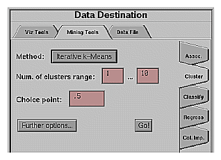
To run iterative k-means, you select three parameters: a lower bound on the number of clusters (default 1), an upper bound on the number of clusters (default 10), and a choice point (default 0.5). See Figure 16-3. Given these parameters, the algorithm proceeds as follows:
Use the minimum number of clusters for a run of the single k-means algorithm. This will produce an initial clustering.
The next steps are run repeatedly until the maximum number of clusters has been reached:
Find the cluster with the greatest dispersion and split it in half, creating two new clusters. Half of the records in the original cluster will be distributed to one of the new clusters and the other half will be distributed to the other new cluster. Recompute the centers of the new clusters based on the data they contain.
If there are any records which are closer to the center of a different cluster than that they are currently in, those records are moved to the closer clusters. The cluster centers are then recomputed based on the new data in each cluster. This is the same as step 4 of the single k-means method. As in the single k-means algorithm, this step is repeated until either no records need to be moved or until it has been run the maximum number of times allowed, as determined by the maximum iterations parameter (default 20).
This process has the effect of producing a range of clusterings between the minimum and maximum numbers of clusters.
The final clustering you are presented with is determined using the choice point parameter (default 0.5) as follows:
Each clustering is evaluated by measuring the average dispersion of each cluster. As the number of clusters increases, the average dispersion always decreases. However, it does not decrease uniformly. The choice point selects the desired degree of dispersion, measured as the proportion from the dispersion of the minimum number of clusters to the dispersion of the maximum number of clusters. The clustering with a measured dispersion closest to this value is chosen as the final clustering. Note that a choice point of 1.0 will always pick the maximum number of clusters, and a choice point of 0.0 will always pick the minimum.
Clusters are named based on their derivation during the splitting process. The initial clustering (based on the minimum number of clusters) is named using sequential numbers, just as in single k-means. Every time a cluster is split, the two new clusters are given the name of the split cluster, but with an “A” or a “B” appended. For example, the cluster named “2-B-A” was derived from cluster 2 in the initial clustering, and was split twice. We built three clusters using the single k-means algorithm with all default options except that we set the attribute weight for iris_type to zero.
When a clustering model is built, you will be presented with the following display of statistics in the status window:
This example is from the iris dataset, available in /usr/lib/MineSet/data.
Result of clustering: ----------------------------------------- Overall root-mean-squared distance from record to centroid: 0.216 +- 0.0928 RMS distance from records to each centroid: Cluster 1: 0.2306 +- 0.09484 Cluster 2: 0.1921 +- 0.09932 Cluster 3: 0.2247 +- 0.08058 Model saved as iris.cluster |
The numbers are measures of the dispersion of each cluster, as well as the overall excellence of fit of the clustering, dispersions from clusterings based on different datasets or different numbers or different numbers of clusters are not immediately comparable.
The k-means clustering algorithm relies on computing the distance between records and the center of a cluster. Each column in the data is treated as a separate dimension in a multi-dimensional space of all records. By default, each column in the data has an equal influence on the final distance. However, you may change the influence of each column, or attribute, by specifying Attribute Weights in the Clustering Options dialog box for clustering, see Figure 16-4.
The attribute weight of a column is a value greater than or equal to zero, which determines the column's influence in the distance computations of the clustering algorithm. Setting an attribute's weight to 1 gives it an average influence. Setting it to 2 gives it the influence of two copies of exactly the same column. Setting it to 0 causes the column to have no effect on the clustering (the clustering proceeds as if you had removed the column from the data before running clustering). Attribute weights need not be integral and may be less than one.
To set attribute weights, first click on the Further options button in the main clustering panel. The top portion of the Further Options dialog box (illustrated in Figure 16-4) shows the current attribute weights, which all default to 1. To change one or more weights, select the column(s) whose weights you wish to change (use Shift-click to select or deselect a range, and Ctrl-click to select or deselect more than one value at once). Now type the new weight value into the Selected weights field. Finally, click the Set button and the selected weights will change to the new value. You may select and set all weights at once using the Select All button.
You will need to adjust attribute weights to help discover a more understandable clustering. Guidelines for weighting are:
String or enum type columns with large numbers of values should generally get low weight (often 0). While such columns will heavily skew the clustering if used by the algorithm, they can help explain the clustering later.
If you have detected several columns which correlate strongly, adjust the weights so that the TOTAL WEIGHT of this set of columns is 1. Otherwise these columns may excessively drive the clustering.
Since distances between categorical (string or enum) columns tend to be greater, it is often useful to give them lower weights than real-valued columns.

-
Clustering gives the opportunity to weight the value of each attribute in the dataset differently. See “Using Attribute Weights” for more information about this option.
-
This metric determines the way in which distances between records and cluster centers should be measured. The default choice is Euclidean distance, which measures distance along a straight line in multidimensional space, with one dimension per column in the data. The popup menu provides an alternate choice, Manhattan. Manhattan distance is computed by adding the distance along the axis of each dimension. This metric gets its name from the way one traverses street blocks in Manhattan: it is not possible to go straight from point A to point B because travel may only proceed along paths parallel to the axes (streets).
Max. # Iterations
This option sets a limit on the number of passes through the dataset the clustering algorithm may use. More specifically, it limits the number of runs of Step 4 in the single k-means algorithm. See the section on the k-means method.
Random Seed
Different random seeds will result in different starting points for the initial cluster centers. See the section on the k-means method.
-
Like most mining tools in MineSet, Clustering supports record weights. This option allows you to specify a column (which must have a numerical value) which will specify the weight of each record in the data.
-
If this box is selected, the designated weight column will also be used as a normal attribute by the clustering algorithm. If this box is unchecked, the designated weight column will not be used as an attribute; it will also disappear from the attribute weights section (it is given an implicit weight of zero).
There are six ways to start the Cluster Visualizer:
Use the Tool Manager to configure and start the Cluster Visualizer. (See Chapter 3 for details on most of the Tool Manager's functionality, which is common to all MineSet tools; see “Working in Cluster Visualizer Main Window” for details about using the Tool Manager with the Cluster Visualizer.)
Double-click the Cluster Visualizer icon, which is in the MineSet page of the icon catalog. The icon is labeled clusterviz. Since no configuration file is specified, the start-up screen requires you to select one by using File > Open.
Double-click the Cluster Visualizer icon on your Silicon Graphics desktop. The startup screen requires you to select a data file by choosing File > Open.
Starting the Cluster Visualizer without specifying a configuration file displays the copyright notice and license agreement for this tool. Only the File and Help pulldown menus can be used. For the main window to be fully functional, open a configuration file by choosing File > Open.
If you know which configuration file you want to use, double-click the icon for that configuration file. This starts the Cluster Visualizer and automatically loads the configuration file you specified. This works only if the configuration filename ends in .clusterviz (which is always the case for configuration files created for the Cluster Visualizer using the Tool Manager).
Drag the configuration file icon onto the Cluster Visualizer icon. This starts the Cluster Visualizer and automatically loads the configuration file you specified. This works even if the configuration filename does not end in .clusterviz.
Start the Cluster Visualizer from the UNIX shell command line by entering this command at the prompt:
clusterviz [ configFile ]
configFile is optional and specifies the name of the configuration file to use. If you don't specify a configuration file, you must use File > Open to specify one.
The Cluster Visualizer requires the following files:
A data file consisting of rows of tab-separated fields. This file is easily created using the Tool Manager (see Chapter 3).
You can generate data files by extracting data from a source (such as a database) and formatting it specifically for use by the Cluster Visualizer. Data files have user-defined extensions (the sample files provided with the Cluster Visualizer have .clusterviz.data extension)
A configuration file, describing the format of the input data and how it is to be displayed. The Tool Manager can create this file (see Chapter 3), or you can use an editor (such as jot, vi, or Emacs) to produce this file yourself.
Configuration files must have a .clusterviz.extension. When starting the Cluster Visualizer, or when opening a file, you must specify the configuration file, not the data file.
Cluster Visualizer illustrated in Figure 16-5 bears a resemblance to Statistics Visualizer (StatViz) with its box plots and histograms. Unlike in StatViz, the box plots are arranged in rows and columns. ClusterViz shows one row for each attribute in the data, and one column for each cluster. At the top of each cluster is a pane containing the name of the cluster. There is one additional column with the title “population”. This column displays statistics for the dataset as a whole and is equivalent to a StatViz view of the data.
Clusters are named based on the mode used to create them. Clusters created using single k-means are numbered sequentially. Clusters created using iterative k-means are numbered according to the process used to create them. In this example the clusters are simply numbered sequentially. The algorithm has no way of detecting what the clusters represent, and human interpretation is required. Each box plot shows statistics about data from a single column, including the minimum, maximum, mean, median, and two quartiles (25th and 75th percentiles). These values are shown as lines, and the standard deviation is shown as a value.
The order in which attributes are displayed in the Cluster Visualizer window is significant; by default, attributes are displayed in order of importance for discriminating between the clusters (this is the same importance ordering as shown in the Evidence Visualizer). Clicking on the pane containing the name of a cluster will redisplay the attributes in order of importance for discriminating that cluster from all others. Clicking on the pane containing “population” will restore the default ordering.

The Cluster Visualizer has three pulldown menus, labeled File, View and Help. These are similar to menus in the Evidence Visualizer (see“Pulldown Menus” in Chapter 13.)
The following example shows a case in which clustering might be useful. This example is associated with a sample dataset provided with MineSet. It shows how to work with the Clustering mining tool, and explains the different outcomes and options.
The cars dataset is relatively simple, dealing with familiar concepts of horsepower, vehicle weight, and time required to reach 60 mph.
In working with the Cluster Visualizer window, when you select cluster 1, that cluster controls the priority ordering of attributes represented by the bar charts and histograms. The order of attributes in other clusters is based on cluster 1. For example, if you click on cluster 1, the attribute importance is cylinders, weight, then miles per gallon. This ordering of importance is a controlling cluster only as far as the visualization goes. You can compare the same row across the other clusters to see how that attribute differs from cluster to cluster. When you select cluster 2, you see a differentiation in the order of attributes at a lower level. In this case, origin is more important, then cylinder, then horsepower, then miles per gallon.
The Cluster Visualizer provides an easy-to-use basic visualization of the clustering. However, it is not the only way to visualize clustering. An example of transferring the results of clustering into a display using the Scatter Visualizer is shown in MineSet 2.5 Tutorial.