This chapter discusses the features and capabilities of the Option Tree inducer. This chapter provides an overview of this tool and discusses methods for using it to generate Option Tree classifiers. The Option Tree Visualizer's functionality is the same as for Decision Trees and was described in Chapter 11. Finally, it lists and describes the sample files provided for this tool.
 | Note: It is assumed that you have read Chapter 10, “MineSet Inducers and Classifiers,” and Chapter 11, “Inducing and Visualizing the Decision Tree Classifier” before proceeding with this chapter. |
An Option Tree classifier assigns each record to a class. The underlying structure used for classification is a Decision Tree, as described in Chapter 11. Figure 12-1 shows an Option Tree where the goal is to predict for the cars dataset the origin of a car built in the 1970's or early 1980's (the origin points being the U.S., Japan, or Europe). Option Trees extend a regular Decision Tree classifier by allowing Option Nodes. An Option Node shows several options that can be chosen at a decision node in the tree. For example, in Figure 12-1, the root is an option node with five options:
cubicinches
cylinders
weightlbs
mpg
brand
Option nodes serve two purposes:
They enhance comprehensibility of the factors affecting the determination of class label by showing several choices that can be made. Instead of using a single attribute at a node, an option node provides you with several options. When flying over the tree, you can choose to follow an option that
you believe is easier to understand, or
you believe is better for predictions based upon your previous experience, or
you select based on the error estimate
In the cars dataset shown in Figure 12-1, you can fly down the cylinders subtree because it has few values, or you can fly down to the weightlbs subtree because its estimated error is lower (1.53). Note that error estimates are only estimates; generally, if the error difference between two options is less than twice their mean standard deviation, then statistically the errors are not different.
They reduce the risk of making a mistake by averaging the votes made by the options below. Every option leads to a subtree that can be thought of as an “expert.” The option node averages these experts' votes. Such averaging can lead to a better classifier with a lower error rate.
In the cars dataset, shown in Figure 12-1, the root node has an estimated error rate of 0.76%, which is lower than any of its children! Note that while brand might seem like a “giveaway” attribute for this task, the training set might not contain all brands (in fact, it does not contain all of them). For an unseen brand, the Decision Tree guesses the majority class (U.S.) and makes two errors. However, when there are other options, they are averaged, and, indeed, the error is reduced.

Option Trees, however, have two disadvantages:
The time necessary to build an Option Tree under the default setting is about 10 to 15 times longer than that needed to build a Decision Tree.
The Tree Visualizer file that is created is more complex, containing 10 to 15 times as many nodes.
Run the Option Tree inducer on your dataset to determine whether the advantages in comprehensibility and error rates justify the longer induction time. You might gain additional insight as to which attributes to remove or use when building a Decision Tree.
An Option Tree classifier is induced (generated) automatically from data. The data, which is made up of records and a label associated with each record, is called the training set (see Chapter 10, “MineSet Inducers and Classifiers”).
The Option Tree inducer requires a training set, as described in the “Training Set” in Chapter 10. Files are generated by extracting data from a source (such as a MineSet ASCII or binary file, or a table in an Oracle, INFORMIX, or Sybase database). To apply the generated classifier, you should have a dataset of records with the attributes used by the classifier, except that the label need not be present.
There are two ways to run the Option Tree inducer:
From the Tool Manager.
Connect to the server and select a data source (see “Choosing a Data Source” in Chapter 3). Enter the filename. For the example shown here, the filename entered would be /usr/lib/MineSet/data/cars.schema as the filename. You'll see several attributes in the Data Transformation panel. Verify that origin is shown as the discrete label. Select the Option Tree inducer, and ensure you have selected the Classifier & Error mode. To run the Inducer, click Go!.
From the command line.
To induce an Option Tree classifier from the command line, refer to Appendix I, “Command-Line Interface to MIndUtil: Analytical Data Mining Algorithms.”
To access the options for configuring the Option Tree inducer, select the Mining Tools tab on the Data Destination panel (Figure 12-2). From the tabs at the right, select Classify. Ensure that the inducer you select is Option Tree. Your selections in the Mode and Inducer menus determine the options available in the Further Inducer Options menu (Figure 12-3). After you have made your selections in these menus, click Go! to run the inducer, which, in turn, creates the classifier.
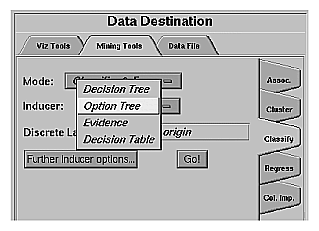
The Discrete Labels menu provides a list of possible discrete labels. Discrete attributes (binned values, character string values, or a few integers) have a limited number of values. You should select a label attribute with few values; for instance, two or three (see “Training Set” in Chapter 10). If there are no discrete attributes, the menu shows No Discrete Label, and the Go! button is disabled. You then must create a discrete attribute by binning or adding a new column using the Tool Manager's Data Transformations panel.
If you have installed the multiprocessor version of MineSet, it is possible to compute tree-based algorithms in parallel whenever a branch contains over 1000 records. Each node on the tree estimates the best possible split on the corresponding level, and these tasks are performed in parallel. The maximum number of threads that a program can spawn is determined automatically by default. You can control the number of threads changing the parallelization mode in the Preferences panel of Tool Manager (see “The File Menu” in Chapter 3). Parallelization may cause memory fragmentation, causing the largest data sets that can be computed in parallel to be smaller than the largest data sets that can be computed on a uniprocessor.
The generated classifier is named with the prefix of the session filename (as determined in Tool Manager) with the suffix -odt.class. By default, all classifiers are stored on the server in the file_cache directory, which defaults to mineset_files. These classifiers can be used for future classification of unlabeled records; that is, they can be used to predict the labels for unlabeled datasets (see “Applying a Model” and “Backfitting in Error Estimation” in Chapter 10).
Selecting Further Classifier Options causes the Further Inducer Options dialog box to appear. This dialog box consists of four panels:
The top panel indicates the choices you made in the Tool Manager's Data Destination panel.
The second pane from the top lets you set the loss matrix and the weight attribute. See “Loss Matrices: Not All Mistakes Were Created Equally” and “Record Weighting: Not All Records Were Sampled Equally” in Chapter 10.
The bottom-left panel lets you specify further Inducer Options.
The bottom-right panel lets you specify the Error Estimation Options (unless the mode you chose in the Data Destination panel was Classifier Only, in which case this area is empty). The options shown in this panel depend on the type of Error Estimation you chose (see “Error Estimation” in Chapter 10).

To fine-tune the Option Tree induction algorithm, you can change any of the options for Decision Trees described in Chapter 11. In addition, the following new options are provided (see Figure 12-3).
-
This integer, which defaults to 5, restricts the maximum number of options that may be created at the root. While the inducer might not allow this number of options because other attributes are inferior, many natural datasets will have many good attributes that could be chosen.
-
This integer, which defaults to 2, defines the amount by which the number of options decreases at every level. With the default of 5 for Max # root options, it implies that there are at most three options (5-2=3) for the second level of decision nodes. The third level of decision nodes is restricted to a single option (3-2=1). Levels further down are similarly restricted to a single option.
-
This ratio determines when to exclude attributes as options. When the inducer gives a fitness score to each attribute, it chooses the best attribute as well as other attributes that might also be good as options. The fitness ratio determines how good those other options must be, to be chosen. A factor value of f implies that to be considered an option, an attribute must rank at least (1-f)*b, where b is the score for the best attribute. A fitness ratio of 1 picks all the attributes (so the limiting options described above are reached if there are attributes on which to split). A fitness ratio of 0 causes a regular Decision Tree to be created (no option nodes).
The time to induce an Option Tree is closely related to the number of option nodes created. Because option nodes usually are created near the top (where they are most useful for both comprehensibility and error reduction), a good approximation for the time to induce an Option Tree is: the number of options created that have no children options times the time to build a Decision Tree. Under the default setting, the root node can have up to five options, and each child can have up to three options. The total options then can be up to 15 (3 times 5). If the option Max # root options is increased to 6, the number of options then is limited by 48 (6*4*2); if it is increased to 7, the number of options is then limited by 105 (7*5*3). Keeping the Max # root options to 5, but changing the decrease to 1, limits the options by 120 (5*4*3*2). The expected induction time for the last example, thus, is two orders of magnitude longer than for a regular Decision Tree. Decreasing the Min fitness ratio option usually results in fewer options than the limiting factor, thus reducing induction time.
The Tree Visualizer's main window shows the Option Tree. The navigation is the same as for decision trees. One feature that is very useful for option trees is clicking the right mouse button on an option node. This presents the list of children, which are the options.
Note that:
The left-most option would have been the only option chosen by the Decision Tree inducer. As you go right, the options are ranked in decreasing order by the fitness scoring. Sometimes, it is interesting to see that the fitness scores do not necessarily match the test-set error shown. This is expected, as the inducer is using a non-perfect scoring function. The test-set estimate also has natural variability: the larger the test-set, the more accurate the estimate.
The option node can have a different error rate than every one of its children. Because the option node averages the children's predictions, its error rate can be different. In some cases, its error is strictly lower than that of every child, showing that averaging helps.
The distribution of instances (shown in bars) at every child of an option node is exactly the same as that of the option node itself. This is because there was no decision made by the option node: options are being presented as children.
The following examples show cases in which the Option Tree inducer can be useful. Each of these examples is associated with a sample data file provided with MineSet. By running the inducer, you can generate the -odt.treeviz files described below. The text describing the scenario and goal for each task is described in “Sample Files” in Chapter 11. Here we describe the specific advantages and disadvantages of Option Trees for several of the example datasets.
| Note: The data files, which have a .schema extension, are located in /usr/lib/MineSet/data on the client workstation. The classifier visualization files, which have a -odt.treeviz extension, reside on the client workstation in /usr/lib/MineSet/treeviz/examples. |
The Option Tree for this dataset shows that total day charge, total day minutes, and customer service calls are all good attributes for the root: they all have approximately the same estimated error rate. You can choose to fly down to one subtree or another, based on your preferences and understanding of the data. Note that while the right subtree starts with customer service calls, the second test is on total daily charge or total daily minutes (as the root's left option). However, because a split already occurred on an attribute, the thresholds are different.
The Option Tree for this dataset shows several good attributes for the root, including: cubic inches, cylinders, weight lbs, mpg, and brand. Note that the root has a lower estimated error rate than any of the children.
This is an example where Option Trees seem to be performing worse than Decision Trees. The root for the Decision Tree shows 6% error and the root for the Option Tree shows 8% error, so it seems that Option Trees perform worse. Be cautioned about making inferences regarding the error rates:
The standard deviation of the error estimate is fairly high: 3.88% and 3.39%. A rule of thumb in statistics is that if the difference is less than two standard deviations, the difference is not statistically significant at the 95% confidence level. A difference of 2% is not larger than even a single standard deviation; hence, the classifier error rates are not statistically different at the 95% confidence level
For small files (Iris has 150 records), different random seeds give different results. For example, changing the seed to 3 improves the Option Tree classifier's error from 8% to 4% without changing the Decision Tree classifier's error rate (remember to reset the seed). This does not imply that a more accurate classifier has been generated, rather that the error estimate is not stable. Because only 50 records are used for testing, each mistake is 2%. The difference between 4% and 8% is making two more mistakes.
For small files (Iris has 150 records), use the “Estimate Error” option in MineSet. It results in better estimates that have narrower confidence intervals. When you run this mode, the status window shows that the Decision Tree classifier has an estimated error of 4.67% +/- 1.73%, and the Option Tree classifier has an estimated error of 4.00% +/- 1.61%. The difference is not significant in this case either, but the Option Tree is slightly superior.
Even if the error rate is higher for Option Trees, they might be (and usually are) better at assigning probability estimates. For this dataset, the estimated mean squared error for Decision Trees is 3.94; for Option Trees it is 3.67 (although the difference is not significant at the 95% confidence level).
The Option Tree for this dataset shows that all five options chosen at the root have zero error rate estimates. Looking at the result, you might prefer the left option (bruises) because it is as accurate but is easier to measure than odor (the root test of the induced Decision Tree). You might want to remove odor and gill size, then build a regular Decision Tree that turns out to be just as accurate (0% estimated error rate).
Note, however, that removal of a root option to have a sibling option selected by the Decision Tree might not necessarily result in the same accurate classifier that is shown in the Option Tree. The removed attribute might have been used lower down in the tree. For example, removing brand from the cars dataset significantly increases the error rate, even though four out of five options do not use it at the root.
This dataset behaves very similarly to the Iris dataset. The Option Tree has the same error rate as the Decision Tree. Under “Estimate error,” the cross-validated estimate shows that it is slightly better than the Decision Tree (but not significantly so at the 95% level) both on error rate and on mean squared error.
The error rate for Option Trees is slightly lower than that for Decision Trees, both for Classifier & Error and for Estimate Error; however, the difference is not significant (at 95%).
The error rates for this dataset are very low (less than 1%), but this is because most people who were tested for hypothyroid (95%) did not suffer from it. If we use a loss matrix that attempts to avoid false negatives (by penalizing by 100 a prediction of negative when the actual value is hypothyroid), we can see that the loss for Option Trees is significantly lower than that of Decision Trees: 182 versus 523 (total), or 0.17 versus 0.5 (per record). This difference is significant at the 95% confidence level.
For this dataset, the Option Tree is slightly more accurate than the Decision Tree; however, looking at the root options, you might notice that it chooses left 1,2, and right 1,2,5. Given the background knowledge that attributes closer to the boundary can be more important, you might want to exclude the option split on right 5. After updating the maximum number of root options to 4 (down from 5), the error rate increases from 5.65% to 6.59%. This might be surprising, given that the root no longer uses right 5 as an option; another effect of changing the number of root options from 5 to 4 was to also reduce the number of options that appear further down the tree (because of the decrease parameter). This caused the individual error rates for each of the other 4 subtrees to increase. Still, the option tree's error rate is significantly better (at the 95% confidence level) than the Decision Tree error rate of 7.06% +/- 0.79%.