This chapter provides an introduction to classifiers and the algorithms that build them, called inducers. MineSet provides three inducer-classifier pairs:
Decision Tree
Option Tree
Evidence
The information in this chapter is equally applicable to all the MineSet classifiers and inducers. The chapter consists of two parts: the first part introduces the basic concepts, and the second part details how to apply those concepts via the Tool Manager.
Detailed descriptions of the MineSet inducers and classifiers are provided in Chapter 11, “Inducing and Visualizing the Decision Tree Classifier,” Chapter 12, “Inducing and Visualizing the Option Tree Classifier,” and Chapter 13, “Inducing and Visualizing the Evidence Classifier.”
A classifier predicts one attribute of a set of data, given several other attributes. For example, if you have data on customers of a telecommunications company, a classifier can be generated to predict whether the customer will churn (leave the company) given information such as whether the customer has voice mail, an international plan or not, and how much time they spend on the phone. The attribute being predicted is called the label, and the attributes used for prediction are called the descriptive attributes.
MineSet can build a classifier automatically from a training set. The training set consists of records in the data for which the label has been supplied. For example, you supply a database table with one column for each descriptive attribute (such as the presence of a voice mail plan, the average number of calling minutes per day), and one column for the label (churned or not). An algorithm that automatically builds a classifier from a training set is called an inducer.
When a classifier is generated, MineSet also generates a visualization that can help you understand how the classifier operates. This visualization can also provide valuable insight into the data itself. Once a classifier is generated, it can be used to classify records that do not contain the label attribute. This value is predicted by the classifier.
 | Note: See Appendix K for a list of further readings about classifiers as well as acknowledgements for the datasets used in MineSet sample files. |
Figure 10-1 shows the Decision Tree generated by the Decision Tree Inducer for the churn dataset.
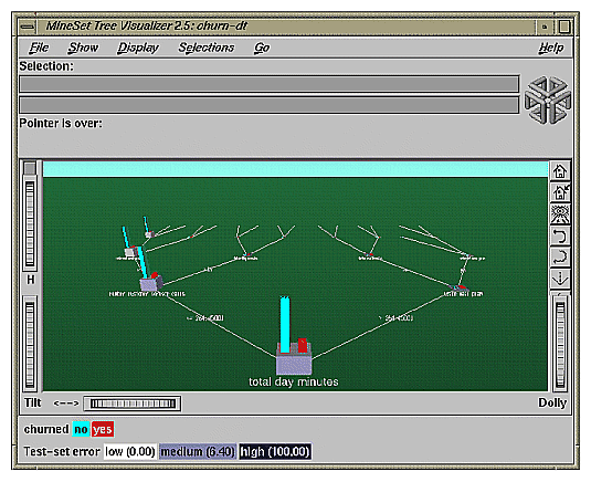
To understand how the Decision Tree classifier assigns a label to each record, look at the attributes tested at the nodes and the values on the connecting lines. In the Decision Tree shown in Figure 10-1, the first test (at the root of the tree) is for total day minutes. There are two branches from this root. If the total day minutes is <= 264.45, the left branch is taken; otherwise the right branch is taken. The process is repeated until a leaf (node with no branches) is reached. The leaf is labeled with the predicted class. The leaf represents a rule that is the conjunction of all tests from the root to the leaf. For example, the right most leaf, labeled No, matches the rule
total day minutes > 264.45 and voice mail plan = yes and
international plan = yes and total day minutes > 276.3
Figure 10-2 shows an Option Tree generated by the Option Tree inducer.
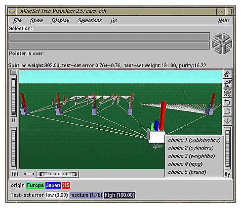
The top node in this figure is an “Option node,” which indicates that several good attributes can be chosen at the root. A Decision Tree Inducer picks the single “best” attribute for each subtree; however, there might be several good attributes on which to split. In such cases, an Option Tree can create option nodes. In the example dataset (Figure 10-2), the task is to predict whether a car is manufactured in Europe, Japan, or the US. The Decision Tree Inducer picks cubic inches for the root. The Option Tree inducer chooses several options: cubic inches, cylinders, weight, mpg, and brand are all good choices for the root.
Option nodes can appear elsewhere besides the root. With the default settings, however, they appear only at the root or one level below the root (after a single test node).
Option Trees usually take 10 to 15 times longer to build than do Decision trees, but they provide two significant advantages:
Comprehensibility — Option nodes let you see several likely options. Instead of having to settle for a single attribute, option nodes let you choose from several. When you fly over the tree, you can choose to follow an option that you believe is easier to understand or that you believe is better for predictions based on your background knowledge of the problem.
Accuracy — In many cases, Option Trees are more accurate (have lower error-rates) than Decision Trees. Option Trees classify by letting each option “vote” for each label value, then average the votes. This is similar to having a series of “experts,” each one attempting to predict the label based on a different main criterion. The option node averages all these experts' votes. Just as distributing stock investments reduces the risk, using a mixture of options usually results in a more stable, less risky classifier.
Figure 10-3 shows the evidence information generated by the Evidence Inducer.
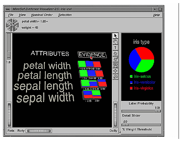
The right window of the screen shows the distribution of the classes in the training set. The left side shows rows of cake charts, one for each attribute. For every value of an attribute in the data, there is one chart matching it in the row for the attribute. Given a record with an attribute value corresponding to a chart, the chart represents how much evidence the classifier “adds” to each possible label value. For example, in Figure 11-3, a record with total day minutes < 175 shows much evidence for the No label value, and little evidence for the Yes label value. After evidence is accumulated from all the attributes, the label value with the most evidence is predicted.
An inducer is an algorithm that builds a classifier from a training set, which consists of records with labels. The training set is used by the inducer to “learn” how to construct the classifier, as shown in Figure 10-4.
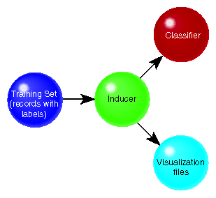
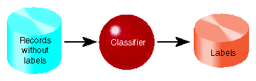
Once the classifier is built, its structure can be visualized or used to classify unlabeled records, as shown in Figure 10-4 and Figure 10-5.
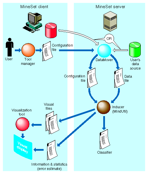
Running inducers can be a CPU- and I/O-intensive process. For this reason, the MineSet inducers run on the MineSet server, rather than on the MineSet client (see Figure 10-6).
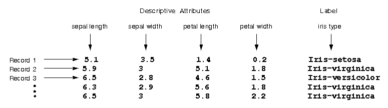
Inducers require a training set, which is a table containing attributes, one of which is designated as the class label. The label attribute type must be discrete (binned values, character string values, or a few integers). The number of possible values for the label attribute should be small, preferably two or three values. Let's look at an example where the goal is to classify the type of an iris flower (iris-setosa, iris-versicolor, or iris-virginica) given as descriptive attributes its sepal length, sepal width, petal length and petal width. Figure 10-7 shows several records from a sample training set for this problem.
Once a classifier is built, it can classify new records as belonging to one of the above classes (see Figure 10-5). These new records must be in a table that has all the attributes used by the classifier with the same name and type as they were in the training set. The table need not contain the label attribute. If it exists, it is ignored during classification.
After building a classifier, you can apply it to records to predict their label. For example, if you built a classifier for predicting iris type, you can apply the classifier to records containing only the descriptive attributes, and a new column is added with the predicted iris type.
In a marketing campaign, for example, a training set can be generated by running the campaign at one city and generating label values according to the responses in that city. A classifier can then be induced and campaign mail can then be sent only to people who are labeled by the classifier as likely to respond, thus saving mailing costs.
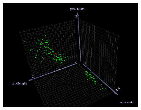
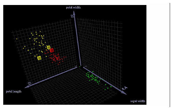
As an example of using mining tools for ensuring data quality, after building a classifier you can apply it to the training set in order to identify records that are mislabeled by the classifier. Such records might warrant closer investigation. Perhaps they are “noise,” or they might yield special insights. If, for example, you have a Decision Tree for the iris dataset induced using the Classify Only mode, by applying the classifier, you get a new column (iris type_1) containing the predicted labels. You can then add a column that is defined as type int with the expression (iris type != iris type_1). The new column has a 1 whenever the classifier misclassifies, and a zero when it correctly classifies. Figure 10-8 shows a Scatter Visualizer plot of the data where the new column is mapped to color with the colors set such that green is 0 (OK) and 1 is red (error). By looking at the plot, it is possible to determine where mistakes are being made.
Another alternative is to define the new column as a float with the expression
(iris type != iris type_1) + 0.01. The Scatter Visualizer can then be used with the original label mapped to color, and this new column mapped to size. Incorrect predictions are shown as big cubes; correct predictions are shown as small cubes (see Figure 10-9).
When a classifier is built, it is useful to know how well you can expect it to perform in the future (what is the classifier's error-rate). Factors affecting classification error-rate include:
The number of records available in the training set.
Since the inducer must learn from the training set, the larger the training set, the more reliable the classifier should be; however, the larger the training set, the longer it takes the inducer to build a classifier. The improvement to the error-rate decreases as the size of the training set increases (this is a case of diminishing returns).
The number of attributes.
More attributes mean more combinations for the inducer to compute, making the problem more difficult for the inducer and requiring more time. Note that sometimes random correlations can lead the inducer astray; consequently, it might build less accurate classifiers (technically, this is known as “overfitting”). If an attribute is irrelevant to the task, remove it from the training set (this can be done using the Tool Manager).
The information in the attributes.
Sometimes there is not enough information in the attributes to correctly predict the label with a low error-rate (for example, trying to determine someone's salary based on their eye color). Adding other attributes (such as profession, hours per week, and age) might reduce the error-rate.
The distribution of future unlabeled records.
If future records come from a distribution different from that of the training set, the error-rate probably will be high. For example, if you build a classifier from a training set containing family cars, it might not be useful when attempting to classify records containing many sport cars, because the distribution of attribute values might be very different.
The two common methods for estimating the error-rate of a classifier are described below. Both of these assume that future records will be sampled from the same distribution as the training set.
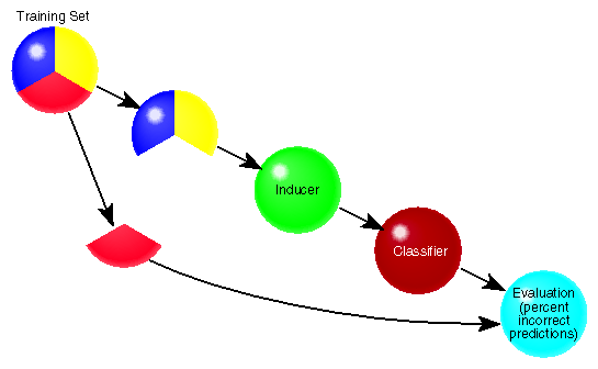
Holdout: A portion of the records (commonly two-thirds) is used as the training set, while the rest is kept as a test set. The inducer is shown only two-thirds of the data and builds a classifier. The test set is then classified using the induced classifier, and the error-rate or loss on this test set is the estimated error-rate or estimated loss. Figure 10-10 shows this error estimation method.
This method is fast, but since it uses only two-thirds of the data for building the classifier, it does not make efficient use of the data for learning. If all the data were used, it is possible that a more accurate classifier could be built.
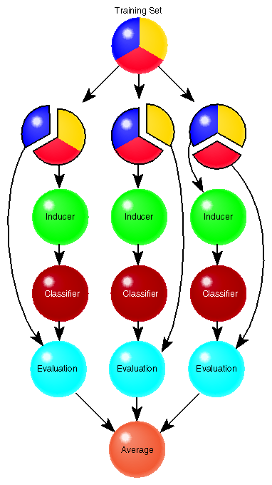
Cross-validation: The data is split into k mutually exclusive subsets (folds) of approximately equal size. The inducer is trained and tested k times; each time, it is trained on all the data minus a different fold, then tested on that holdout fold. The estimated error-rate is then the average of the errors obtained. Figure 10-11 shows cross-validation with k=3 (note that the default value is k=10).
Cross-validation can be repeated multiple times (t). For a t times k-fold cross-validation, k*t classifiers are built and evaluated. This means the time for cross-validation is k*t times longer. By default, k=10 and t=1, so cross-validation takes approximately 10 times longer than building a single classifier.
Increasing the number of repetitions (t) increases the running time and improves the error estimate and the corresponding confidence interval.
You can increase or decrease k. Reducing it to 3 or 5 shortens the running time; however, estimates are likely to be biased pessimistically because of the smaller training set sizes. You can increase k, but this is recommended only for very small datasets.
Generally, a holdout estimate should be used at the exploratory stage, as well as on datasets of over 5,000 records. Cross-validation should be used for the final classifier building phase, as well as on small datasets.
An inducer builds a classifier, which has two parts:
Structure — For Decision Trees and Option Trees, the structure is the shape of the tree. For evidence, the structure is the number of bins for every attribute and the thresholds if the attribute is numeric.
Probability estimates — Each part of the structure estimates the probability of each class. These estimates are commonly based on the counts of training records at different points in the structure. For Decision Trees, the probabilities are determined by the weight of records at the leaves. For the Evidence classifier, the probabilities are determined by the conditional probabilities for every attribute value or range.
Backfitting a classifier with a set of records does not alter the structure of the classifier, but updates the probability estimates based on the given data. Backfitting is useful for several reasons:
A structure can be built from a small training set, then backfitted with a big dataset to improve the probability estimates in the structure. Backfitting is a faster process than inducing the classifier's structure.
When holdout error estimation is used, a portion of the data is left out for testing. Once the classifier structure is induced and the error estimated, it is possible to backfit all of the data through the structure, which can reduce the error of the final classifier. When counts, weights, and probabilities are shown in the classifier's structure, they reflect all the data, not just the training set portion.
When using drill-through from the visualizers, you can see data corresponding to the weights shown, which reflect the whole dataset. If backfitting is not used, the weights shown represent only the training set.
Confusion matrices give a more detailed picture of the errors made by a classifier. Instead of simply analyzing the number of correct and incorrect predictions, the confusion matrix shows the type of errors being made.
Figure 10-12 shows a confusion matrix for a Decision Tree that was induced on the iris dataset.

The two axes represent:
the class values predicted by the classifier, and
the actual class values given in the test set (holdout set).
Entries on the diagonal are correct predictions. Entries off the diagonal indicate incorrect predictions. This representation shows that iris-versicolor and iris-virginica are frequently confused, but iris-setosa is always predicted correctly.
When the cost of making different types of mistakes is uneven, it is frequently useful to understand the type of errors that are being made (see loss matrices below).
| Note: The confusion matrix shows the errors made on the test set; thus, it represents the expected true distribution of errors in an actual situation if the underlying distribution of the data does not change significantly. The confusion matrix in MineSet is computed prior to backfitting and is the same whether or not backfitting is applied. |
A lift curve is a graph that plots the cumulative weight of the records from a specified label value as a function of the weight of all the records. The order in which the records occur determines the slope of the curve. Typically, a lift curve plots the difference between randomly ordered records and records sorted based on a classifier's predictions.
For example, in telecommunications, it is valuable to be able to predict which customers are likely to switch providers (churn). In the dataset churn, about 13.5% of the customers are likely to switch provider. Figure 10-13 shows the lift curve obtained by using a Decision Tree classifier on this dataset.
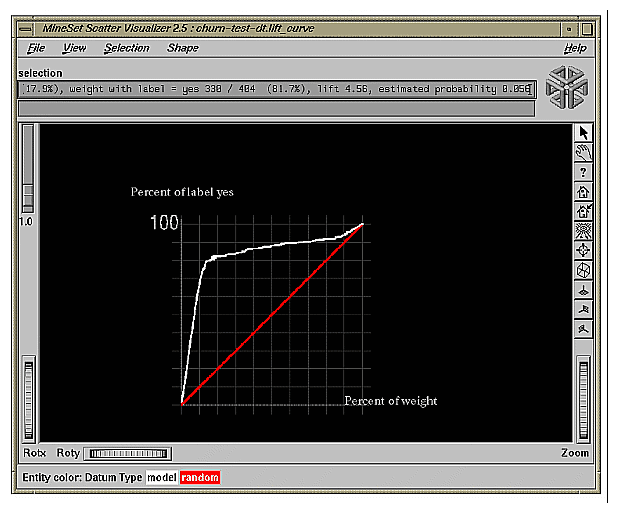
The X axis shows the number of records sampled; the Y axis shows the number of records corresponding to customers who churn. The lower curve (red) shows the number of customers expected to churn given a random ordering of the records. The upper curve (white) shows the percentage of customers that churn when ordered according to the classifier's score (probability estimate) for each record. Records representing customers that the classifier identifies as most likely to churn appear first; those less likely to churn appear last. The lift that the classifier ordering provides can be seen by the difference between the classifier curve and the random curve.
If some action should be taken before customers churn, it should be prioritized according to the classifier's score. If the action costs money (for example, an operator contacting the customer or a mailing), lift curves can help identify a cutoff point that maximizes returns.
| Note: The lift curve shows lift on the test set; thus, it represents the expected true lift in actual situations if the underlying distribution of the data does not change significantly. The lift curve in MineSet is computed prior to backfitting and is the same whether or not backfitting is applied. |
A learning curve is a graph that shows the error of the classifier generated by an inducer as a function of the number of records used to create the classifier. Typically, the more records used to generate the classifier, the lower its error.
A learning curve is created by generating the specified number of classifiers for each of the points on the curve. Each classifier is generated using a random sample of the records, and its error is estimated using the rest of the records (those not used for training).
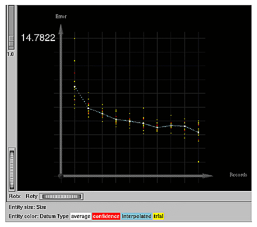
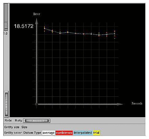
Figure 10-14 shows a learning curve for the Decision Tree Inducer on the churn dataset. Figure 10-15 shows a learning curve for the Decision Tree Inducer on the adult dataset with the label set to gross income binned at $50,000 (so one class is gross income less than or equal to $50,000 and the other class is gross income >$50,000). The X axis shows the number of records used for training the inducer; the Y axis shows the error. The graph consists of four type of points:
The yellow points are the actual error estimates taken from the runs.
The white points are averages.
The blue points interpolate between the white points.
The red points show a 95% confidence interval about the average based on actual error estimates for each run.
The more runs that are requested, and the bigger the test set (portion used to test), the smaller the confidence interval. The error is generally reduced as more records are used for training.
We can see that for the churn dataset, the error continues to decrease as the training set size grows, while for the adult dataset, there is little advantage to training on the whole dataset. The third point represents about 13,000 records and has an estimated error of 16.96%, while the last point represents about 44,000 records and has an estimated error of 16.85%.
A small sample might suffice for most of the study, with the full data used only for the final runs. In many cases, a small sample can result in a sufficiently accurate classifier, with the error reducing only slightly if the number of records is increased (diminishing returns). Once a learning curve is seen, the desired sampling point can be determined, and the “sample” transformation in Tool Manager can be used to generate a sample of this size (see “The Sample Button” in Chapter 3). Small samples reduce the time needed to build a classifier and make the knowledge discovery process more interactive.
MineSet supports several advanced options for all inducers. These let you take into account different costs for making mistakes and to take into account an experimental design that has a non-uniform sampling process (that is, some parts of the true population are sampled more heavily than others). Another option lets you create more complicated classifiers which may have better accuracy, at the expense of added compute time.
Suppose you are trying to classify mushrooms as poisonous or edible. Classifying a mushroom that is actually edible as poisonous might cost you $2, since you are not eating it; however, classifying a poisonous mushroom as edible (that is, eating it) might incur a $10,000 operation.
Figure 10-16 shows a confusion matrix for the mushroom dataset with the Decision Tree Inducer when only a ratio of 0.1 (10%) was used for a training set.
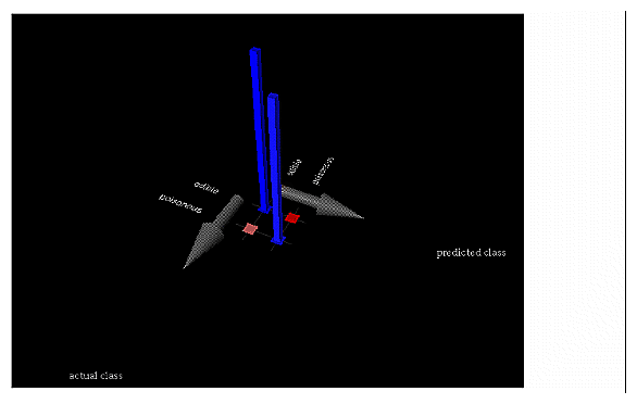
Eight records, representing poisonous mushrooms, were classified as edible (0.1%); 15 records, representing edible mushrooms, were classified as poisonous (0.2%). 3793 edible mushrooms and 3496 poisonous mushrooms were correctly classified. While the error-rate for the classifier is only 0.31% (less than one percent), our estimated loss would be $10000*8 + $2*15 = $80,030.
Figure 10-17 shows a confusion matrix for the same dataset, but with the Decision Tree Inducer run using a loss matrix representing the above costs. The new classifier is very conservative and makes no mistakes in classifying a poisonous mushroom as edible; but it makes 1558 mistakes (1543+8) in classifying edible mushrooms as poisonous. The total estimated loss we would incur is thus $10000*0 + $2*1558 = $3116, only 3% of the cost of the classifier that did not take losses into account.
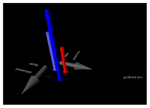
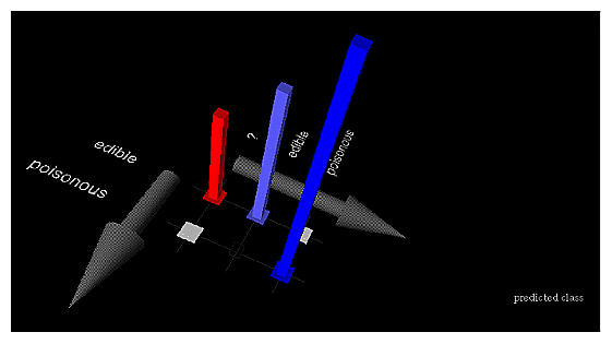
Loss matrices also allow predicting unknown (null values), which are shown as question marks (?). For example, suppose it costs us $1 to ask an outside expert whether a mushroom is poisonous or edible. In that case, some classifications result in an unknown prediction. Running the Decision Tree Inducer yields the confusion matrix shown in Figure 10-18, where there are 1551 unknowns, and only 15 edible mushrooms are classified as poisonous. The overall cost is thus $10000*0 + $1*1551 + $15*2 = $1581
Figure 10-18. Confusion Matrix for the Mushroom Dataset With Loss Matrix Allowing Unknown Predictions
 |
Note that loss matrices are based on probability estimates made at the leaves of the tree. For reliable estimates:
Raise the "split lower bound" in Further Options of Decision Trees and Option Trees from the default value to a higher value (for example: 5). In general, the larger and noisier the training set size, the higher this value should be.
Use large training sets. You might need large training sets to get reliable estimates when the costs are not as extreme as in this example.
Use Option Trees. While they do not always help, they usually provide better probability estimates that tend to reduce the loss. For example, running the above example with $10000 changed to $100 with unknowns not allowed, yields an estimated loss of $1464 for Decision Trees and an estimated loss of $662 for Option Trees.
A Return-on-Investment (ROI) curve is similar to a Lift Curve, but displays accuracy in terms of loss rather than in terms of error; taking into account the Loss Matrix used. The points in an ROI curve are ordered by the expected loss for each record, were they to be labeled by the chosen label value. Similarly, the height of each point in the curve indicates the cumulative profit (inverse loss), rather than the cumulative accuracy (inverse error) of all records up to this point. The expected loss is computed by multiplying entries in the Loss Matrix, under the chosen labels column (see “Loss Matrices,” under “Advanced Options,” below) by the probabilities assigned to the corresponding classes, for the classes by the classifier. Hence, if the classifier is very sure about its prediction, the expected loss will be low, and the record will appear near the left side of the ROI curve.
The idea behind the ROI curve is that the user will take an action for each individual record in the dataset. That action will be the one associated with the chosen label value. For example, in the churn dataset, the action associated with the label Yes, might be to send that person some marketing material. This might stop the person from churning; but the action is costly if done indiscriminately. The peak of the ROI curve shows approximately how much money would have been saved on the test set, if the classifier was used to predict whether or not to send the mailing to a particular person.
Special care needs to be taken when filling out a Loss Matrix for use with a Loss Curve. The column under a certain predicted label determines the resulting ROI curve for that label value. The entries in this column need to represent the expected gain or loss for taking the action associated with that label value, on all of the possible classes. For example, the entry under the column “prediction yes” in churn, under the row “actual value no”, may contain the value 2 to indicate that the cost of mailing a brochure (the action associated with “yes”) to someone who was not going to churn, is 2 dollars. On the other hand, the entry under the column yes, row yes, may have a value of -10 to indicate that a customer was prevented from churning, saving the company ten dollars over the cost of the mailing.
In certain experimental designs, portions of the true population are sampled more frequently than others. For example, while you might want a 1% sample of some population, a small minority that is already 0.1% of the population results in a 0.001% sample, which might be too small (for instance, you might get two people). Record weighting lets you give each record a weight; thus, a subpopulation that was sampled twice as frequently might get a weight of 0.5, while the rest of the population is given a weight of 1.
As another example, a phone company stores all fraudulent phone calls in the dataset, while storing only a small fraction of non-fraudulent calls. By using record weighting, it is possible give each record its true portion of the population.
Finally, some datasets are already aggregated, and the records have a natural “count” associated with them (for example, statistics about cities in the U.S. usually have an associated count of the population). This count attribute can be mapped to weight, which is equivalent to replicating each record by the number of counts.
The semantics of record weighting is that a record weight of 2 is equivalent to two records with a record weight of 1. Floating point weights are allowed.
In some cases, the most important issue in creating a classifier is its error rate. For example, suppose you have analyzed a dataset for churn prediction to a point that you are satisfied with, and are ready to create a classifier that will predict which of your customers are the most likely to churn. At this point, you are no longer interested in visualizing your classifier, since you have a reasonably good understanding of the factors that are involved. You also want to achieve the best classification accuracy possible. In this case, you might want to enable Boosting, which is an algorithm that creates several different classifiers and combines their predictions using a weighted voting scheme. Boosted classifiers often improve classifier accuracy, by focusing the induction process on examples in the data which are harder to model than others.
Boosting will not always increase accuracy, but it often does. Boosted classifiers cannot be visualized, though you can still see confusion matrices, lift curves, learning curves and ROI curves for boosted classifiers. Boosting is a computationally intensive process, often taking 25 times longer to run than the corresponding inducer without Boosting. Backfitting does not work with Boosted classifiers, because of the special way Boosting weights multiple classifiers and the records used to train them.
The theory behind boosting has not been generalized past two-class problems. MineSet 2.5 and later versions, however, allow you to use boosting with labels that have any number of values. Boosting will not always improve the error rate of induced classifiers; this is especially stressed for problems that have more than two label values.
Boosting works by repeatedly assigning new weight distributions to the training set and inducing classifiers on the reweighted sets. The number of times this occurs is limited by the BOOST_NUM_TRIALS option, which can be set using the .mineset-classopt files on the client (see Appendix I, “Command-Line Interface to MIndUtil: Analytical Data Mining Algorithms,”for more information about the .mineset-classopt file). The number of classifiers generated may be lower than this parameter if the training set error rate drops to zero before this many classifiers are generated.
The following section describes the options provided for the classifiers by the Tool Manager.
There are four modes for running an inducer (shown in Figure 10-19).
Classifier and Error
Classifier Only
Estimate Error
Learning Curve
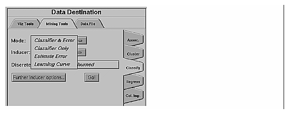
The Classifier and Error mode uses a holdout method to build a classifier: a random portion of the data is used for training (commonly two-thirds) and the rest for testing. This holdout proportion can be set in Further Inducer Options (see “Error Estimation”). This method is the default mode and is recommended for initial explorations. It is fast and provides an error estimate.
The Classifier Only mode uses all the data to build the classifier. There is no error estimation. Use this mode when there is little data or when you build the final classifier.
The Estimate Error mode assesses the error of a classifier that would be built if all the data were used (as with Classifier Only mode). Estimate Error uses cross-validation, resulting in long running times. Cross-validation splits the data into k folds (commonly 10) and builds k classifiers. The process can be repeated multiple times to increase the reliability of the estimate. You can set the number k and the number of times in Further Inducer Options, as explained in “Error Options for Inducers,” below. Use this method when there is little data. The induced classifier is exactly the same as the one induced by the Classifier Only mode.
The Learning Curve mode assesses the effect of training set size on the error of a classifier.
The following options are available to fine tune the error estimation for the inducers. The Error Options available to you depend on the mode you have chosen.
In both Classifier & Error and Estimate Error, you can set a random seed that determines how the data is split into training and testing sets. Changing the random seed causes a different split of the data into training and test sets. If the error estimate varies appreciably, the induction process is not stable.
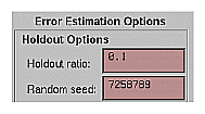
In Classifier & Error (see Figure 10-20), you can set the Holdout Ratio of records to keep as the training set. This defaults to 0.666667 (two-thirds). The rest of the records are used for assessing the error.
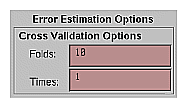
In Estimate Error (see Figure 10-21), you can set the number of folds in cross validation and the number of times to repeat the process.
The Backfit test set option is a checkmark that can be found under Further Options for all inducers when using Classifier & Error mode, and is shown in Figure 10-22. The backfit checkmark is disabled when Boosting is enabled.
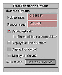
The Display Confusion Matrix option is checkmark under Further Options for all inducers when using Classifier & Error mode is shown in Figure 10-22.
The Display ROI Curve option is a checkmark under Further Options for all inducers when the classifier and Error mode is shown in Figure 10-23. An ROI curve requires a label value to be chosen. An ROI curve is then generated and displayed for that label value.
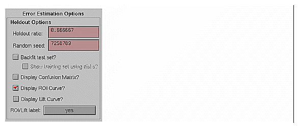
The Display Lift Curve option is a checkmark under Further Options for all inducers when using Classifier & Error mode is shown in Figure 10-22. A Lift Curve requires a label value to be chosen. A lift curve is generated and displayed for that label value.
The Use Loss Matrix option is a checkmark under Further Options for all inducers (See Figure 10-24). The Edit matrix button can then be used to define the loss matrix. To avoid unknowns from being predicted, fill the unknown prediction column with the highest value in the matrix.
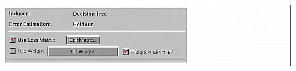
The Use Weight option is a checkmark under Further Options for all inducers (See Figure 10-24). Choose the column for the weight. The Weight is Attribute option determines whether the inducer can use this attribute for classification purposes or not. In certain cases where the weight is a result of a stratified sample that is part of the experimental design, the classifier should not be given access to the weight column as it is not a property of the real-word entity.
Learning Curve is a mode in the Classify menu of the Mining Tools tab. It can be used with any of the inducers. When the Learning Curve mode is selected, the Further Options dialog box lets you specify Learning Curve Options (shown in Figure 10-25), including:
the number of points in the learning curve,
the number of runs per point, and
the number of records to use at the start and end points.
The number of records to use at each intermediate point is calculated automatically.
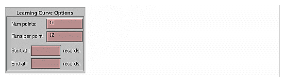
The number of points in the learning curve must be specified; also, it must be greater than or equal to 1. The number of records for the starting and ending points can be specified to allow generating a learning curve for a specific range of the training set. If either of these options are left blank, they are calculated automatically based on the number of points in the learning curve and the total number of records in the training set. This default covers the entire range of the training set. For instance, assume a file containing 80,000 records. If you specified 3 points in the learning curve, the algorithm generates points at 20,000, 40,000 and 60,000 records. Often it is useful to “zoom in” on a smaller range. For example, a learning curve might be generated only for a range of 1000 to 10,000 records.
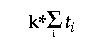
Generating a learning curve takes a significant amount of CPU time. If ti is the time to train an inducer on training set i (where i ranges from 1 to the number of points), and there are k runs per point, the total time is shown below . Increasing the number of runs per point increases the running time proportionally, but improves the estimate of the average. The default value of the number of runs is 3.
 |
The Scatter Visualizer's filter panel can be used to filter some of the data types shown (average points, confidence intervals, interpolated points, or actual trials). For example, you might want to remove the data points for the trials and confidence intervals and show only the averages and interpolated points.
Once you have specified the Classification Options, click OK to have these options take effect and to return to the Data Destination panel. To return to the Data Destination panel without having changes to the options take effect, click Cancel.
After you press Go! in the Data Destination panel, the Status Window at the bottom of the Tool Manager's main window shows the inducer's progress and the output classifier's statistics. It displays specific information for the induced classifier. For example, for Decision Trees it shows the number of nodes, the number of leaves, and the depth of the Decision Tree (Figure 10-26). This information is saved automatically on your workstation under the session file name with a -dt.out, -odt.out, or -eviviz.out extension, depending on whether a Decision Tree, Option Tree, or Evidence Inducer was executed.
For Classifier & Error, the first series of dots represent reading the file, then information about the classifier build progress is shown, then the test set classification progress is shown.
For Classifier Only mode, there is no test set classification phase.
For Estimate Error, the times and folds are shown.
For Learning curves, each average point on the x-axis will be described on a line and each run for that average point will be represented by a dot.
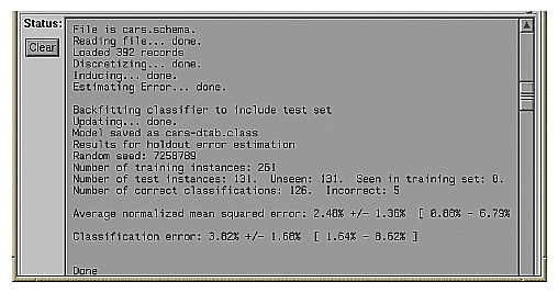
When you have selected the Classifier & Error mode, the Status window contains the following information:
The random seed used to split the data into training and test sets.
The number of records used for training the inducer.
The number of records used for evaluating the resulting classifier; of the test records, how many were seen during training, excluding the label attribute. It is possible to have duplicate records (“seen”) in a dataset; some records can be in both the training and test set. A large value of seen records indicates that there are many duplicate records. If their labels are contradictory, it might be impossible to achieve high accuracy without adding more attributes to the dataset.
The number of correct and incorrect predictions made.
The average normalized mean squared error represents the accuracy of the probability estimates. For each test record, the mean squared error is the square of one minus the probability estimate for the correct label value, plus the sum of the squares of the probability estimates for the other (incorrect) label values. The normalized mean squared error is half the mean squared error, which is a value between zero and one. The average normalized mean squared error is the normalized mean squared error averaged over all the records in the test set by their appropriate weights (weighted average).
The classification error, which is the percent of incorrect predictions.
Both the average mean squared error and the classification error show the standard deviation of the mean and the confidence interval for the mean. This is the range you can expect from the classifier if the data comes from the same distribution. For error estimates (not losses), a more accurate formula than the usual two-standard deviation rule is used.
When you have selected the Estimate Error mode, the Status window contains the following information:
The number of cross-validation folds and times.
The random seed.
The estimated accuracy with standard deviation.
The 95% confidence interval for the estimated accuracy.
The Apply Model button in the Data Transformations panel lets you:
take a previously created classifier and apply it to new data.
test a previously created classifier's performance on the current table.
fit the current table into a previously created classifier's structure.
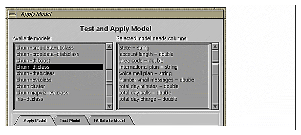
On the top left of this dialog box (Figure 10-27) is a list of all classifiers currently available on the server. If you select a classifier, the right-hand side lists the column names and types required by that classifier. If these requirements match the current table, a message at the bottom states this, and the buttons on the bottom (OK, Run Test, or Fit Data) is activated. If the current table does not have all the columns required for the selected classifier, the message at the bottom states this, the columns that are missing are selected in the list on the right, and the button on the bottom is deactivated.
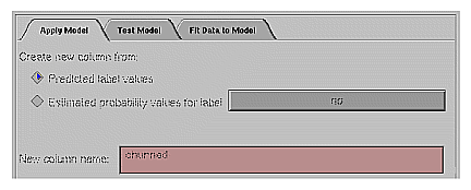
The Apply Model panel is used to apply a previously created classifier to the current table, as shown in Figure 10-28. There are two modes of application for the classifier:
To Predict discrete label values for the records in the current table. For example, if you created a classifier to determine churn, you can use this option to add a column that labels each customer as either likely to churn or not likely to churn.
To generate Estimated probability values for a specified label value. Instead of using the classifier to predict the label value of each record, it is used to estimate the probability that each record has a specified label value (for example, churn = yes). Given the classifier created to determine churn, you can use this option to add a column that indicates the probability that each customer is likely to churn.
The New column name text field lets you specify the name of the new column.
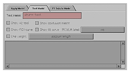
The Test Model panel is used to test a previously created classifier on the current table, as shown in Figure 10-29. The table must contain columns with the names and types required by the selected classifier. Unlike Apply Model, Test Model also requires the table to contain a label column with the same name and type as the label column used when building the classifier.
The Test Model panel has options that lets you
show the confusion matrix of the classifier on the table records
show the lift curve of the classifier for a specified label value
show the ROI curve of the classifier for a specified label value
show a visualization of the classifier with the table used as the test-set (this is only relevant for Decision Tree and Option Tree classifiers)
select an attribute to use as the record weight
The text field at the bottom of the Test Model panel shows the results.
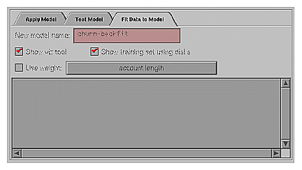
The Fit Data to Model panel is used to fit the data in the current table to a previously created classifier, as shown in Figure 10-30. This produces a new classifier with the same structure as the original one; however, the new one uses the data from the table to update the probability estimates (see “Backfitting in Error Estimation”). Because all of the data from the table is being fit into the structure of the classifier, there is no error estimation. Fit Data to Model cannot be used on classifiers that were built using boosting. Use Test Model to evaluate the performance of the new classifier on a separate test set (disjoint from the fit data).
The Fit Data to Model panel has options that lets you
The following subsections describe how to set special options and the limitations of the inducers.
When the Tool Manager runs an inducer on the server (the MIndUtil program), it passes certain options to the inducers. Not all options are controlled through the Tool Manager GUI. Those options not controlled by Tool Manager take on their default values and can be overridden by setting them in a special file, called .mineset-classopt. Tool Manager prepends this file to the options sent. This file is optional. Tool Manager looks for it first in the current directory, then in your home directory. See Appendix I, “Command-Line Interface to MIndUtil: Analytical Data Mining Algorithms” for more details about the options.
The file should contain one line per option, in the following format:
<OPTION>=<value> |
For example, the special option LOGLEVEL increases the amount of information shown during the induction process. The default of zero shows very little information. Level 1 shows other options and slightly more information. Level 2 and higher show large amounts of information about the induction process. These levels are appropriate only if you have a firm understanding of the induction process. (See Appendix K, “Further Reading and Acknowledgments.”)
Note that these options are not part of the saved session. If you send files to other users, you might have to send this file separately to them.
Three limits and their respective options are as follows:
Discrete attributes are ignored if they have more than 100 values. Discrete attributes with many values are usually inappropriate for classification. For example, first names and street addresses are unlikely to form predictive patterns.
To speed up the induction process, attributes with over 100 values are ignored.
You can override this value by setting MAX_ATTR_VALS to a higher number. For example, your .mineset-classopt file could contain the line
MAX_ATTR_VALS=500
Discrete labels with over 25 values are not allowed by default. Automatically induced classifiers are rarely appropriate for predicting one of a large number of label values. You should limit the label to a few values (preferably two or three). You can override this default limit by setting the option MAX_LABEL_VALS to a higher value in your .mineset-classopt file.
Boosting works by repeatedly assigning new weight distributions to the training set and inducing classifiers on the reweighted sets. The number of times this occurs is limited by the BOOST_NUM_TRIALS option, which can be set by the .mineset-classopt file on the client. The number of classifiers generated may be lower than this parameter if the training set error rate drops to zero before this many classifiers are generated.
There are three further limitations:
Floating point numbers are read into MIndUtil as floats (4 bytes) even if they are represented as doubles (8 bytes) in the database, in the ASCII file, or in the binary file. This limits the precision and magnitude of the representations allowed.
Dates are considered strings. Unless there are few dates, such attributes are usually ignored because of the limit on discrete attributes. You should bin dates before running an inducer.