This chapter introduces predictive modeling and explains how to use MineSet to generate predictive models from datasets. The visualizations generated by MineSet then help you understand how the model operates. Drill through techniques allow you to examine the underlying data. The topics discussed are:
Subsequent chapters show the visualizations and models in greater depth. For greater technical details, refer to the MineSet Enterprise Edition Reference Guide .
MineSet contains a number of analytical data mining algorithms that generate predictive models. A predictive model predicts the value of an attribute called the label, given the value of several other attributes in the record. If there is enough information in the attributes, the model can accurately predict the label. The predicted label refers to the unknown characteristic in a given record. For example, in a credit history dataset, given the values for attributes “age”, “sex”, and “occupation”, the task of a predictive model might be to predict the value of the attribute “credit_risk.”
If you have data where the label is unknown, use predictive modeling, but if you want to visualize data where the label is known, descriptive modeling is more appropriate. MineSet's two types of predictive modeling are classification and regression. Classification predicts discrete values and regression predicts values in a continuous range. Each of these is detailed in subsequent chapters. This chapter discusses processes common to all predictive models.
The MineSet algorithms for generating predictive models depend on the type of attribute that will be predicted. For classification tasks, MineSet's algorithms generate an Evidence model, a Decision Tree, an Option Tree, or a Decision Table. For regression tasks, MineSet generates a Regression Tree.
The following five subsections provide a short introduction to the various types of predictive models that MineSet supports, and illustrate how they may be generated. You can tailor the way the model-generating algorithm works from Tool Manager's Data Destinations pane using the Advanced Options button. For a more detailed technical description of how these options effect the model generators, see the “Inducer Modes in Tool Manager” entry in the MineSet Enterprise Edition Reference Guide .
See Appendix A in the MineSet Enterprise Edition Interface Guide for a list of further readings about individual inducers.
This section shows you how to generate a predictive model called the Evidence Classifier, for more details see Chapter 10, “Modeling and Predicting with the Evidence Classifier and Visualizer.”
To build a predictive model, begin by selecting a dataset using the Tool Manager. See “Starting MineSet” in Chapter 2 for details. This example uses the churn dataset to build models that predict which customers are likely to change telecommunications providers.
In the Tool Manager Data Destinations pane, click the Mining Tools tab.
Click the Classify tab, and make these selections from the popup menus:
Mode: Classifier Only
Inducer: Evidence
Discrete Label: churned (for example)
You are about to induce an evidence classifier to help characterize the customers who are likely to churn. In this case you use all the data to build the model, and don't hold any in reserve for testing the accuracy.
Click Go.
The Status window on the bottom of Tool Manager shows progress and summary information about the induction process. When the induction step is done, the Evidence Visualizer is automatically invoked, showing a visual representation of the model as in Figure 7-1.
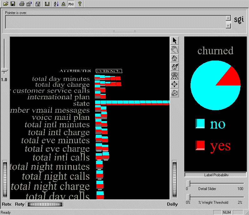
This model shows how well each attribute predicts the value of churn. For an explanation of how to use this model for predictive behavior, see Chapter 10, “Modeling and Predicting with the Evidence Classifier and Visualizer.”
In the previous example you used the Evidence method to induce and visualize the classifier. If you choose the Decision Tree method you can show how various attributes interact, that is, how combinations of attribute values affect the predicted label. With the Decision Tree, how the data is distributed at subsequent nodes (decision points) depends on the decision made at the previous node. In the example shown in Figure 7-2, the root decision point splits on whether the total day minutes attribute is greater than or less than 264.45. This affects the distribution of values at subsequent branches; clearly, higher bars appear on the left of the visualization.
To generate a Decision Tree Model follow the same steps as for the Evidence Model, except when you choose the Inducer on the Classify tab, choose Decision Tree. The task is explained in full in Chapter 8, “Modeling and Predicting with Decision, Option, and Regression Trees.” The result of this method is shown in Figure 7-2. The fact that the distribution of classes in subtrees branching out from the root are different shows that interactions between attributes are significant.
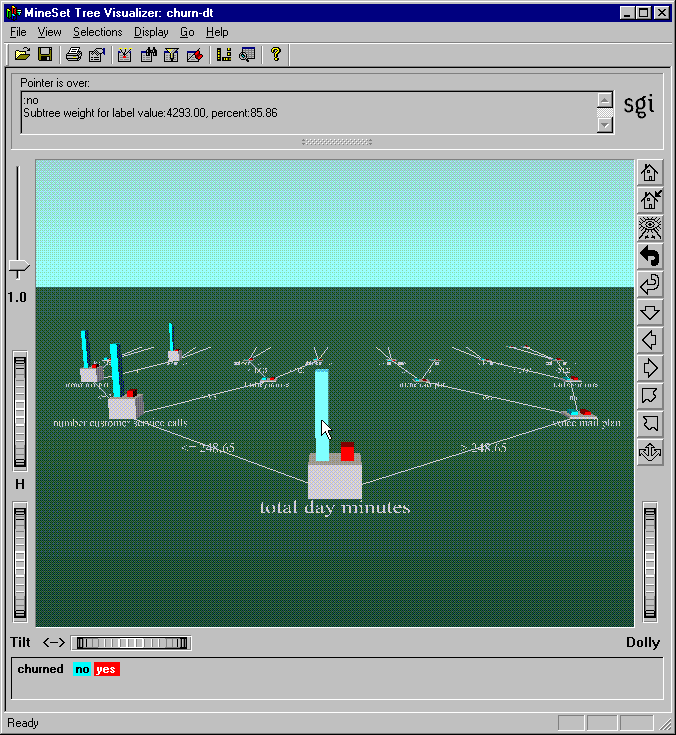
The bars at each node of this decision tree represent the distribution of label values (classes). Placing the cursor over a bar shows the record weight and percentage for that label value in the status area above the display. The height of the base of each node represents the weight (record count if no weighting is used) of the records.
In this example the block that is the root of the decision tree is marked with the label “total day minutes,” indicating that this is the single most important factor in predicting churn—how long these customers talked, with a dividing threshold of 264.45 minutes. The Decision Tree is explained in further detail in Chapter 8, “Modeling and Predicting with Decision, Option, and Regression Trees.”
A Decision Tree Inducer picks the single “best” attribute for each subtree; however, there might be several good attributes on which to split. In such cases, an Option Tree can create option nodes. An Option Tree appears similar to a Decision Tree but is generated by the Option Tree inducer.
The top node is an “Option node,” showing that several good attributes can be chosen at the root. You can set the number of options generated at each option node, representing the best attributes at that point. A branch is then generated for each option. The example shown in Figure 7-3 uses the cars dataset. The Option Tree is explained in further detail in Chapter 8, “Modeling and Predicting with Decision, Option, and Regression Trees.”

In the example dataset (Figure 7-3), the task is to predict whether a car is manufactured in Europe, Japan, or the U.S. The Decision Tree Inducer picks cubic inches for the root. By contrast, the Option Tree inducer chooses several options: cubic inches, cylinders, weight, mpg, and brand as alternative good choices for the root. You can see these choices by clicking the Ctrl key and right mouse button on the root.
Option nodes can appear elsewhere besides the root. With the default settings, however, they appear only at the root or one level below the root.
Option Trees usually take 10 to 15 times longer to build, and are much larger than, Decision Trees, but they provide two significant advantages:
Flexibility—Option nodes let you see several likely options. Instead of settling for a single attribute, option nodes let you choose from several. When you fly over the tree, you can follow an option that is easier to understand or fits your background knowledge of the problem.
Accuracy—Often, Option Trees have lower error rates than Decision Trees. Option Trees classify by letting each option “vote” for each label value, then averaging the votes. This is similar to having a panel of experts, each one attempting to predict the label based on a different main criterion. The option node averages all these experts' votes, resulting in a more stable, less risky classifier.
The Decision Table induces a model that presents correlations between pairs of attributes in a layered hierarchy. Decisions are made by the inducer in the same way as the Decision Tree, but attributes are evaluated across the entire level of the tree rather than on a specific sub-tree. The result is then presented as a hierarchical table rather than a tree. Clicking on the blocks in the visualization shows the details of how the rectangular block called a cake is composed, as shown in Figure 7-4.
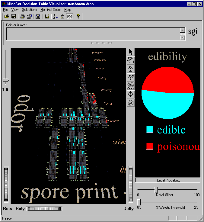
This model shows the label probability in predicting the edibility of mushrooms.
See Chapter 9, “Modeling and Predicting with the Decision Table Classifier and Visualizer,” for a description of how to use the Decision Table.
The Regression Tree Inducer generates a regressor, which is a predictive model similar to the classifier. The difference is that regressors predict labels with values in the continuous range, such as an individual's annual salary. Classifiers predict only discrete values, such as yes or no, or a specific range such as 20-100.

The following example shows you how to generate a regressor, a task that is expanded in Chapter 8, “Modeling and Predicting with Decision, Option, and Regression Trees.”
To build a predictive regressor, begin by selecting a dataset using the Tool Manager. See Chapter 2, “Accessing Data with MineSet,” for details. This example uses the adult dataset.
In the Tool Manager Data Destinations pane, click the Mining Tools tab.
Click the Regress tab, and make these selections from the popup menus:
Mode: Regressor Only
Inducer: Regression Tree
Continuous Label: gross income (for example)
You are about to induce a regressor to help characterize the gross income of adults represented by records in the dataset. In this case you use all the data to build the model.
Click Go.
The Status window on the bottom of Tool Manager shows progress and summary information about the induction process, or you can watch the progress indicator on the dialog box. When the induction step is done, the Regression Tree Visualizer is automatically invoked, showing the model visually as in Figure 7-5. Some datasets take a longer time to generate than others.
You can generate a regressor only for datasets using continuous attributes, that is, with a column containing data in a continuous range. If there are none, you can add a new continuous column from the Tool Manager Data Transformations pane, see “Removing and Adding Columns” in Chapter 3.
The Learning Curve classifier mode is discussed in “Creating a Learning Curve”.
The goal of predictive models is to make predictions, therefore the usefulness of the model is clearly dependent upon the accuracy of its predictions. The accuracy of a model is measured by the error rate. This section discusses the range of MineSet's modes of modeling: Classifier Only using all the data and with no error estimation; and the two common methods for estimating error rate—holdout and cross-validation.
In the holdout method of estimating errors, a section of the dataset (commonly two-thirds) is held out to generate the model. The inducer uses the labels in this training set of data and constructs the model, the rest of the data is used to test the model and estimate the error-rate.
Cross-validation is a method of estimating classifier error that splits the dataset into a certain number of folds, or subsets, (commonly 10), and builds that same number classifiers. The process can be repeated multiple times to increase the reliability of the estimate.
Both holdout and cross-validation methods expect future records to be sampled from the same data distribution as the training set. A more complete discussion may be found in “Error Estimation” and “Cross-Validation” entries in the MineSet Enterprise Edition Reference Guide .
The Classifier Only mode of building the model uses all available data to build the classifier. It is useful when you are not concerned about estimating the error rate of the predictive model, such as when you just want to see the visualization.
Suppose you want a Decision Tree for the iris dataset induced using the Classifier Only mode. This example goes through the entire sequence of building and applying the model. You could find out when the model misclassifies by following these steps:
From the Tool Manager window select a dataset using the File > Open New Data File pulldown menu. Choose the iris.schema dataset.
From the Tool Manager Data Destinations pane, click the Mining Tools tab, then click the Classify tab and choose:
Mode: Classifier Only
Inducer: Decision Tree
Discrete label: iris type
You are using all available data to build a Decision Tree model that determines what attributes distinguish between types of irises.
Click Go to run the Decision Tree. Examine then dismiss the visualization. The created model used all the data. The following steps show you how to evaluate correct and incorrect predictions in such a case.
In the Tool Manager Data Transformations pane click Apply Model. Select iris-dt.class (the iris decision table classifier), and click OK to accept the default New column name iris type_1, which now contains the predicted labels.
Click the Add Column button to create another new column that will identify errors (call the column iris_fault). You can then add a column that is defined as type int with the expression (`iris type' != `iris type_1').
To build the expression, select from the left list, and press the right-pointing arrow, or type directly in the text field.
Click Check Expression, and then click OK. This adds the new column iris_fault, based on iris type_1. The new column has a 1 whenever the classifier misclassifies, and a zero when it correctly classifies.
Verify your results. In the Tool Manager Data Destination pane, click Viz Tools, choose Record Viewer from the Tool popup menu and click Invoke Tool. An example of the result is shown in Figure 7-6.
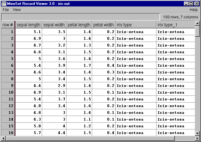
You can then apply your results to a scatterplot so that the new column is mapped to color, with the colors set such that green is 0 (no error) and 1 is red (error). See Chapter 4, “Examining Data with the Scatter and Splat Visualizers,” for examples of the Scatter Visualizer.
Instead of using all the data to build the model, you can hold out part of the data as a training set to induce the classifier. The Classifier and Error mode (MineSet's default mode) automatically partitions the dataset into independent training and test subsets. The proportion of data used as the training set can be changed to fit your requirements.
To see an example of how holdout error estimation applies to a selected dataset, follow these steps:
Start with the iris.schema dataset (see page 129).
From the Tool Manager Data Destinations pane click the Mining Tools tab, then click the Classify tab and choose:
Mode: Classifier and Error
Inducer: Decision Tree
Discrete label: iris type
You are partitioning the iris dataset into two sets. The training set containing two-thirds, the default holdout ratio of records, is used to build the Decision Tree model. The remaining one-third of the records are used to estimate the error rate of the model.
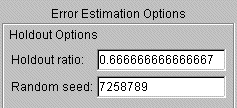
Click the Advanced Options button to vary the holdout ratio of the training set using the text panel shown in Figure 7-7. You may also change the random seed to get different records in the training and test sets. See the glossary entry Random Seed. Dismiss the panel by clicking OK.
Run the Decision Tree inducer by clicking Go.
The error rate of the inducer estimated using the test set (the remaining one-third of the data) is displayed in the status area at the bottom of the main window. You can scroll down to see all the information.
Use cross-validation for building the final classifier or for small datasets. The process used should explain the reason. Cross-validation is a method for getting a more precise estimate of error. In n-fold cross-validation (where n represents any number you care to name and fold is number of subsets into which you divide the data), the dataset is partitioned into n independent subsets. In turn each of these subsets is held out and the remaining n-1 subsets (one less than the number you originally specified) are combined to form a training set. The resulting model is evaluated using the held-out subset. These n independent estimates are then averaged and the data is combined to build the final model. N-fold cross validation takes approximately n+1 times longer than Classifier and Error, or Classifier Only methods.
To apply cross-validation to a selected dataset and set the number of Folds:
From the Tool Manager Data Destination pane, choose the Mining Tools tab and click Classify.
From the Mode popup menu choose Estimate Error to assess the error if all the data were used (as with Classifier Only mode). Running time is likely to be long, since cross-validation is used. Use Estimate Error when there is little data. The induced classifier is exactly the same as the one induced by the Classifier Only mode.
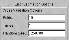
Click the Advanced Options button to change the way the cross-validation operates. In Error Estimation Options (see Figure 7-8), you can set the number of Folds and the number of Times to repeat the error estimation process. Accept any changes by clicking OK.
Run the algorithm by clicking Go.
For a more detailed discussion of Error Estimation, see the its entry in the MineSet Enterprise Edition Reference Guide.
The Learning Curve shows the error of the classifier generated by an inducer in proportion to the number of records used to create the classifier. Typically, the more records used to generate the classifier, the lower its error.
You create a Learning Curve by indicating the range of training set sizes you want to investigate, and the number of times you want to build an inducer at each training set size. To indicate the range of training set size you want to investigate, enter the start (minimum) and end (maximum) number of records and the number of points to examine. Each classifier is generated using a random sample of the records, and its error is estimated using the remaining records (those not used for training).
Start with the churn.schema dataset used on page 122.
From the Tool Manager Data Destinations pane click Mining Tools, then click the Classify tab and choose:
Mode: Learning Curve
Inducer: Decision Tree
Discrete Label: churned (for example)
You will be prompted that the phone number column will not be computed because it contains too many unique values. You can either remove the column or simply click OK.
Click Go.
The process takes a long time because the inducer is generating a classifier for each point on the curve. The status window displays the training size, the number of times the training is being done, and the mean error in each pass.
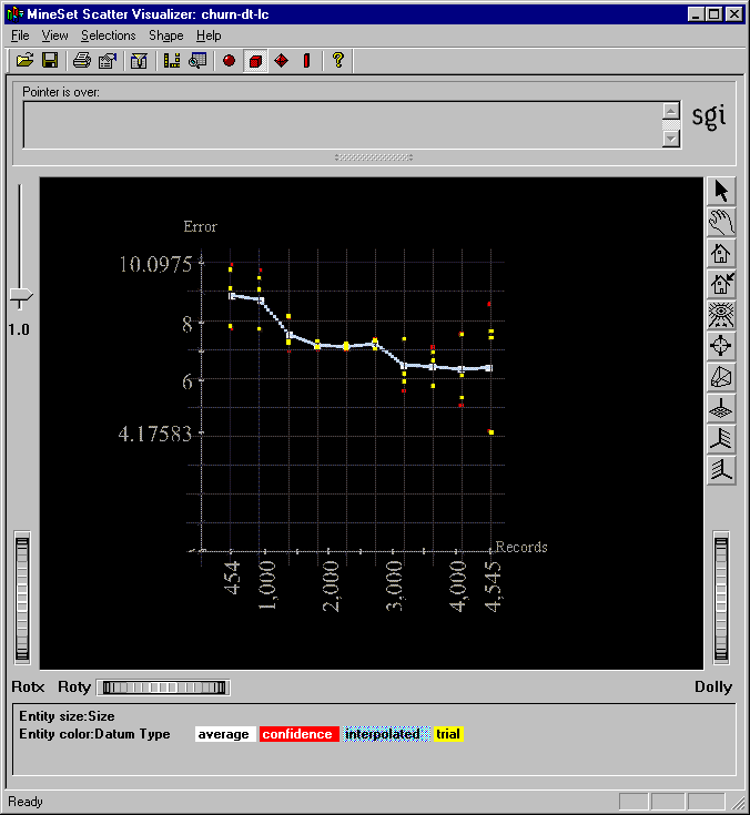
Figure 7-9 indicates the error rate for a given number of records in the churn dataset. If you train on 454 records, there is an error of 9.41%, if you train on almost all the records there is an error of 5.27%. By identifying the point at which the error rate no longer decreases, you can determine the number of training records needed to produce a classifier with the desired error rate. In this case it appears that training on 3,000 records is sufficient. You can pick a sample size based on a point on the learning curve with reasonable accuracy.
The graph shows four types of points:
The yellow points are the actual error estimates taken from the runs (number of times the algorithm runs).
The white points are averages.
The blue points (sometimes resembling a blue line) interpolate between the white points.
The red points show a 95% confidence interval about the average, based on actual error estimates for each run.
By default the algorithm uses all the records to build the learning curve, but you can specify other modes:
Using the previous Learning Curve, Decision Tree, and churned selections from the Tool Manager Data Destination pane, click Advanced Options.
From the Advanced Options dialog box, you can specify these Learning Curve Options (Figure 7-10)
Number of points in the learning curve—must be greater than one.
Number of runs per point.
Number of records to use at the start and end points.
The number of records to use at each intermediate point is calculated automatically.
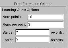
If either the range or the number of points is left blank, it is calculated automatically based on the number of points in the learning curve and the total number of records in the training set. This default covers the entire range of the training set. For instance, assume a file containing 80,000 records. If you specify 3 points in the learning curve, the algorithm generates points at 20,000, 40,000 and 60,000 records. Often it is useful to “zoom in” on a smaller range. For example, a learning curve might be generated only for a range of 1,000 to 10,000 records.
Increasing the number of runs per point increases the running time proportionally, but improves the estimate of the error. The default value of the number of runs is 3.
A learning curve may be generated for any inducer. You can run with the defaults or quantify the points in the curve, number of runs to make, or the range of records. Table 7-1 shows the effect of certain choices on a learning curve.
Table 7-1. Actions for Learning Curve Results
To achieve this result: | Do this: |
|---|---|
Reduced confidence interval (greater accuracy) | Increase number of runs. Increase size of test set. |
Speed processing | Use small sample (see “Sampling Data”). |
For detailed information on the operation of inducers, refer to the “Inducer” entry in MineSet Enterprise Edition Reference Guide .
After building a predictive model, you can apply it to other records to predict their label. For example, if you built a classifier for predicting iris type, you can apply the classifier to records containing only the descriptive attributes, and a new column will be added with the predicted iris type.
Models generated by MineSet are saved in your designated server directory. For example, churn-dt.class is a decision tree model generated from the churn dataset. You can apply this classifier to another data table you specify. After you have built the model using the Decision Tree for this example, follow these steps:
In the Tool Manager Data Transformations pane click the Apply Model button.
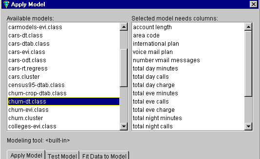
From the Test and Apply Model dialog box (Figure 7-11), select a model in the “Available models” pane. The right-hand pane then lists the column names and types required by that classifier.
If these requirements match the current table that is loaded in memory, the buttons on the bottom of each tab (OK, Run Test, or Fit Data) are activated. If the requirements do not match, the columns that are missing are selected in the list on the right, and the bottom buttons are deactivated.
After you have selected the model you wish to apply:
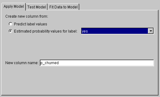
In the Test and Apply Model dialog box, click the Apply Model tab (Figure 7-12) and select one of the following:
Predicted label values: adds a column to predict, for example, if a customer will churn. The new column lets you see how well the model predicts when used on new data.
Estimated probability values: estimates the probability that each record has a given label value. Select the available values from the popup menu. This adds a column that estimates the probability of correctness as a numerical value.
Enter a name for the new column in the text field, for example, p_churned to represent the probability of a customer churning.
Click OK.
To graphically display the model as a table of columns, from the Tool Manager Data Destination pane, click Viz Tools and from the Tool popup menu choose Record Viewer, and click Invoke Tool.
The labeled columns churn and p_churned are displayed, allowing you to match predictions and results.
Applying a model might be used in a marketing campaign, in which a model was generated from running the campaign in one city and generating a column recording (label) values according to the responses in that city. The model might be applied and campaign mail can then be sent only to people in another city who are labeled by the classifier as likely to respond, thereby saving mailing costs.
The next several chapters describe various ways of looking at data, and include an indication of the particular strengths of each visualizer. Accordingly, you may find yourself beginning with Record Viewer to look at raw untransformed data, progressing through the Statistics or Histogram Visualizer, and then searching for important columns using the Column Importance tool in preparation for achieving a useful visualization of known data with the Scatter, Splat, or Map Visualizer.
If you have no hypotheses from which to start, you may want to start by clustering and let that method drive your knowledge discovery.
If you are ready to test and apply a model, and to determine model accuracy, several approaches can be found in Chapter 11, “Refining Predictive Modeling.”