This chapter builds on concepts developed in previous chapters, using the Tool Manager to examine the cost of making errors in classification, and to fit data mining operations to real-life needs. MineSet's advanced options for inducers allow you to improve accuracy, to compensate for the cost of making mistakes, and to determine the stage at which it is pointless to continue investing in a project. The sections in this chapter are:
The screen illustrations may be viewed in color using the online version of this guide (available from the Help menu).
The model you have previously developed can be checked for accuracy in different ways. A few methods have been discussed in “Evaluating a Predictive Model”. This section continues the discussion with methods of verifying the model using different sources. If you do not presently have a model, return to Chapter 7, “Understanding Predictive Modeling,” for help in creating one.
If you have a model created at an earlier time, MineSet allows you test it on data you are currently working on, using the Test Model facility. The columns in the dataset must contain the same names and types as those used when creating the model.
Unlike Apply Model (described in “Applying a Predictive Model” in Chapter 7) Test Model requires that the table also contain a label column with the same name and type as that used when building the model. The reason for this is that the test must work from data for which you have the correct answer. The test file is assigned a default name with the suffix -test, such as iris-test.
The following example creates a test file from the iris dataset. Once you have logged in to the server, select your dataset (the example file is MineSet\data\iris.schema, in the directory where MineSet was originally installed).
To test a model on the current dataset, follow these steps:
In the Tool Manager Data Transformations pane, click the Apply Model button.
From the Test and Apply Model dialog box, click the Test Model tab.
Select the name of the model from the list of available models that appears at the top of the dialog box (for example iris-dt.class) and the default test filename appears (Figure 11-1).
If your current table is missing any columns, those column names are highlighted in the “Selected model needs columns” list on the right. Choose another model or restore the missing columns. The Test Model panel gives you these options:
Table 11-1. Test Model Panel Options
Selection
Action
Test name
Shows the name of the test file, which you can change.
Show viz tool
Shows a visualization of the classifier with the table used as the test set.
Show confusion matrix
Shows confusion matrix of model based on table records. See “Displaying a Confusion Matrix”.
Show ROI curve
Shows ROI curve of model using the specified label value. See “Finding Marketing Benefits Using a Return on Investment Curve”.
Show lift curve
Shows lift curve of model using the specified label value. See also “Assessing Models with the Lift Curve and ROI Curve”.
ROI/Lift label
Displays popup menu of available label values.
Use weight
Select an available attribute from the popup menu by which to weight the records. See also “Weighting Records” in Chapter 3.
Click Run Test. The text field at the bottom of the Test Model panel shows the results, and the visualizer options you selected are displayed.
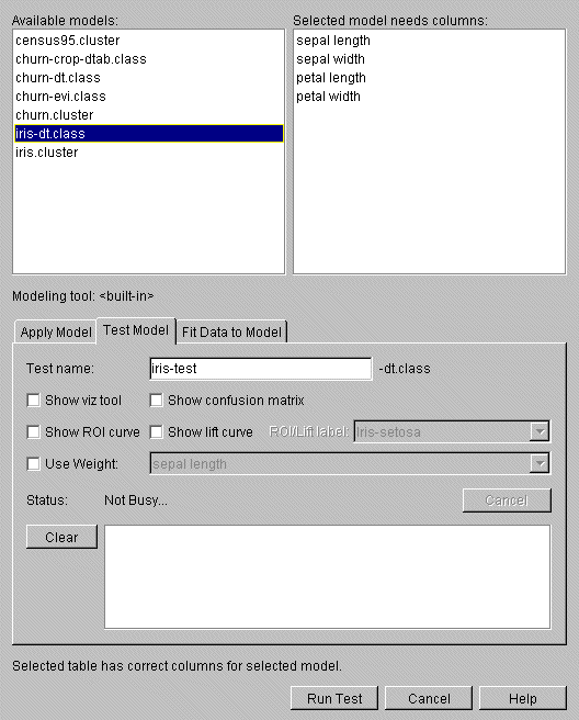
In this case, the entire dataset of iris.schema is run on a previously created model, iris-dt.class, and four errors are noted on 150 test instances.
When you have fresh data, use the Fit Data to Model panel (Figure 11-2) to fit the data in the current table to a previously created model. This produces a new model with the same structure as the original one; however, the new one uses the data from the table to update the probability estimates (see “Backfitting in Error Estimation”). Because all of the data from the table is being fit into the structure of the model, there is no error estimation. Fit Data to Model cannot be used on models that were built using boosting. See “Improving Accuracy with Boosting” below. If you want to evaluate the performance of the new model on a separate test set (disjoint from the fit data), use the Test Model facility.
To fit data to an existing model, follow these steps:
In the Tool Manager Data Transformations pane, click the Apply Model button.
From the Test and Apply Model dialog box click the Fit Data to Model tab. (Figure 11-2). Fit Data to Model options appear in Table 11-2.
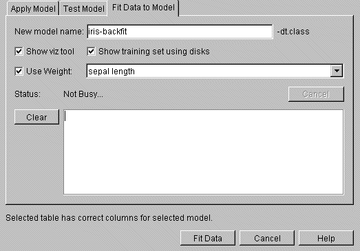
The Fit Data to Model panel (Figure 11-2) gives you these options:
Table 11-2. Fit Data to Model Options
Selection | Action |
|---|---|
Show viz tool | Shows a visualization of the new model (only for tree-based models). |
Show training set using disks | Sets disks to indicate proportion of training set data in visualization. |
Use Weight | Select an attribute from the popup menu to use as record weight. |
When you backfit a model with a set of records, you update the probability estimates, you do not alter the structure of the model. Backfitting is similar to fitting data to a model, a mode that defaults to using backfitting. Backfitting is useful when:
You build a model structure from a small training set and backfit it with a large dataset. This is often quicker than inducing the larger model structure.
You need greater accuracy. When counts, weights, and probabilities are shown in the model's structure, they reflect all the data, not just the training set portion.
To enable backfitting:
In the Data Destinations pane of the Tool Manager window, click the Mining Tools tab.
Click the Classify tab.
Choose the Classifier and Error mode, and click the Advanced Options button to bring up the Advanced Options dialog. Click the Backfit test set check box under Error Estimation Options. The check mark is disabled when Boosting is enabled.
In some cases error rate is the most important criterion in choosing a model, so you might want to enable boosting. Boosting is an algorithm that creates several different models and combines their predictions using a weighted voting scheme. Boosting improves model accuracy by focusing the induction process on examples in the data that are harder to model than others. However, boosted models cannot be visualized.
To activate boosting on any selected model:
In the Tool Manager Data Destinations pane, click Mining Tools.
Click the Classify tab.
From any mode click the Advanced Options button to bring up the Advanced Options dialog. Click the Boost (no viz) check box in the Inducer options section.
Boosting does not always increase accuracy, but it often does. Boosted models cannot be visualized, though you can still see confusion matrices, lift curves, learning curves and ROI curves for boosted models. Boosting is a computationally intensive process, often taking 25 times longer to run than the corresponding inducer without boosting. Boosted models may not use backfitting.
 | Note: Although the theory behind boosting has not been generalized past two-class problems, MineSet allows you to use boosting with labels that have any number of values. Boosting is less likely to improve the error rate in these cases. |
Boosting works by repeatedly assigning new weight distributions to the training set and inducing models on the reweighted sets. See the MineSet Enterprise Edition Reference Guide for further information on boosting.
When you find errors in classification, it is helpful to know in what way the classifier is becoming confused, and the extent of loss this confusion entails. MineSet provides two complementary matrices to answer your questions: the Confusion Matrix and the Loss Matrix.
Suppose you are trying to classify mushrooms as poisonous or edible. Classifying a mushroom as poisonous might cost you $2 (the cost of the mushroom). Classifying a poisonous mushroom as edible however, might land you in the hospital with a $10,000 hospital bill (optimistically). The MineSet Confusion Matrix and Loss Matrix features are designed for handling such situations, and can give a detailed picture of errors and incorrect predictions.
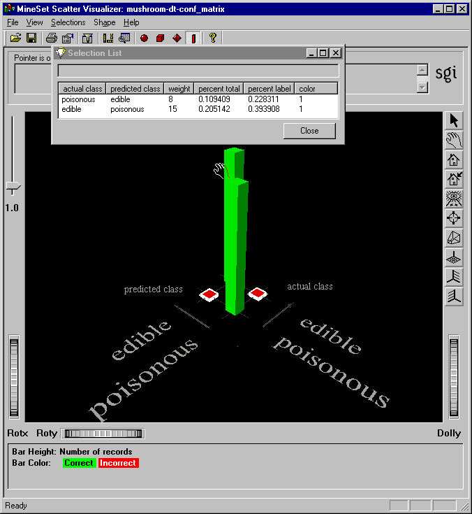
Figure 11-3 shows a Confusion Matrix for the mushroom dataset with a Decision Tree trained on 10% of the dataset, considerably less than the recommended training set. See Chapter 7, “Understanding Predictive Modeling,” for details.
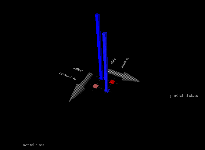
Eight records representing poisonous mushrooms were classified as edible (0.1%); 15 records representing edible mushrooms were classified as poisonous (0.2%). The remaining 3793 edible mushrooms and 3496 poisonous mushrooms were correctly classified. While the error rate for the model is only 0.31% (less than one percent), the estimated loss based on the example in previous paragraph is $10000*8 + $2*15 = $80,030.
Confusion Matrices give a more detailed picture of errors made by a model, by displaying a visualization of the type of errors being made. The two axes represent the predicted class values and the actual class values given in the test set (holdout set). The Confusion Matrix is computed prior to backfitting. The following section shows how to use a Confusion Matrix that follows the above scenario.
For this example use the Tool Manager window to open the data file mushroom.schema, and explore confusions in classifying mushrooms as edible or poisonous. This file is in the MineSet\data directory, in the location where MineSet was initially installed.
From the Tool Manager Data Destinations pane, click the Mining Tools tab; then click the Classify tab and make selections from these popup menus:
Mode: Classifier and Error
Inducer: Decision Tree
Discrete Label: edibility
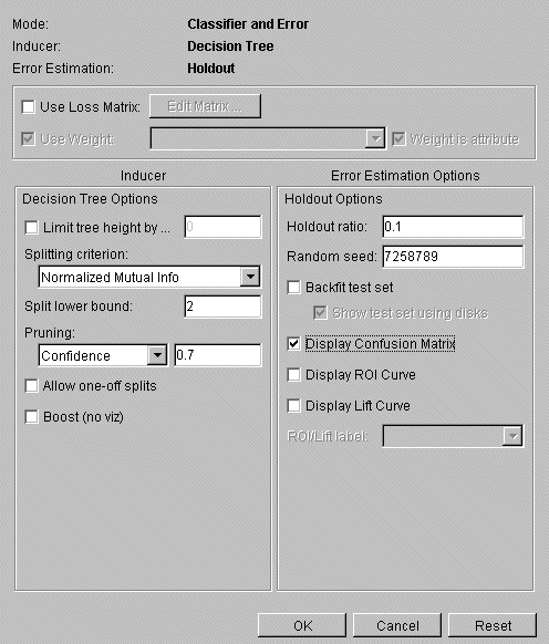
Click Advanced Options and the Classifier Advanced Options pane shown in Figure 11-4 appears.
In the Error Estimation Options pane, change Holdout ratio to 0.1, turn off Backfit test set, click the check box at Display Confusion Matrix, then click OK.
You are reducing the size of the training set in order to cause the classifier to make mistakes for demonstration purposes. A typical training set would be much larger.
Click Go on the Tool Manager Data Destinations pane.
When the Decision Tree visualization appears, dismiss it and examine the Confusion Matrix shown in Figure 11-5. The Confusion Matrix displays where the classifier makes mistakes in classifying. From this you can construct a Loss Matrix based on what you now know about the data, to make certain kinds of errors less tolerable than others.
The display shown in Figure 11-5 indicates that using this reduced training set, eight poisonous mushrooms were misclassified as edible, or 0.1% of total. Click on a selection in the visualization, then choose Show Values from the Selections menu of the Tool Manager to see the Selection List table.
This section explains how a Loss Matrix may be used to reduce the more costly types of classification errors. The example continues the scenario from the previous section, using the mushroom dataset, a decision tree inducer, and classifying for the label edibility.
Dismiss the Confusion Matrix display with File > Exit and return to the Tool Manager window.
On the Mining Tools tab in the Data Destinations pane, click Advanced Options to open to the Classifier options pane.
In the second section of the pane, click Use Loss Matrix; wait briefly.
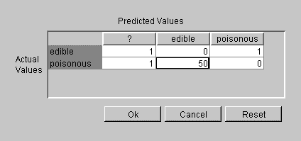
Click Edit Matrix to weight the cost of making errors. A Loss Matrix window similar to that shown in Figure 11-6 appears.
Set these values across the Actual Values rows of the Loss Matrix, reading from left to right as shown in Figure 11-6:
edible: 1—0—1
poisonous: 1—50—0
This weights the cost of classifying poisonous mushrooms as edible 50 times more expensive as the reverse.
Click OK to set the Loss Matrix values settings, and Go to run the classifier.
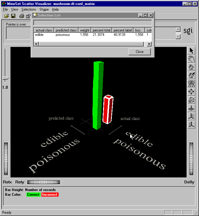
The new classifier is very conservative; no mistakes are made in classifying a poisonous mushroom as edible. On the other hand, 1558 mistakes are made in classifying an edible mushroom as poisonous. Using the figures of the cost of mushrooms ($2 each) versus hospital stay($10,000), the new estimated loss incurred is $10,000*0 + $2*1,558 = $3,116, only 3% of the cost of the classifier that did not take losses into account. Figure 11-7 shows the resulting Confusion Matrix.
For more information on Error Estimation, see the MineSet Enterprise Edition Reference Guide .
When a business embarks on a course of action, it is often helpful to anticipate gains or losses before changing course or abandoning a project. MineSet provides an opportunity to gauge a probable outcome, and to make changes before events have significant impact. Two methods of doing this are with the Lift Curve and the Return-on-Investment (ROI) Curve.
A lift curve is a graph that shows the difference between a random ordering of records and an ordering produced by a model in predicting a particular label value. For example, when you create a model to predict which customers are likely to churn, you may want to target customers who are likely to churn before they actually churn. The lift curve helps accomplish this goal. This example uses the churn dataset.
A lift curve plots the number of records from 0 to 100% on the X axis and the number of records corresponding to customers who have a given label value (Churn=yes in this case) on the Y axis.
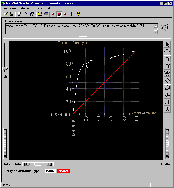
Two curves are shown on the graph in Figure 11-8. The lower curve (red) shows the number of customers expected to churn given a random ordering of the records. The upper curve (white) shows the percentage of customers who churn when placed in order according to the model's score (probability estimate) for each record. Records representing customers whom the model identifies as most likely to churn appear first; those less likely to churn appear last. The advantage that the model ordering provides can be seen by the difference between the model curve and the random curve.
In building this lift curve, a selected model is applied to the test set. In the example, a specified segment of the dataset is used for training. Then the induced model is run on the remainder of the dataset.
To generate a lift curve on any selected model:
In the Tool Manager Data Destinations pane, click the Mining Tools tab.
Click the Classify tab.
Choose the Classifier and Error mode and Decision Tree inducer.
Click Advanced Options, and from the Classifier options popup menu, click the Display Lift Curve check box under Error Estimation Options. Choose a label value (yes) from the ROI/Lift label popup menu.
Click OK to accept the inducer options and dismiss the dialog box.
Click Go.
The process may take some time. Dismiss the Decision Tree. The resulting lift curve shows the details of any selected point in the selection window under the task bar. Move the pointer along the white (model) line, and click at various points to see the lift and percentage of customers with churn=yes. Look for the knee of the curve, in this example, where the estimated probability of the classifier is 0.056. This is the point at which the return on investment in sending incentives to customers that may churn diminishes rapidly. The next step is to apply the classifier to the full dataset (see “Classifying Using All Your Data” in Chapter 7).
A Return-on-Investment (ROI) curve is similar to a Lift Curve, but displays accuracy in terms of loss rather than in terms of error; depending on how you weight your Loss Matrix (see “Defining a Loss Matrix”). If the model is sure about its prediction, the expected loss will be low, and the record appears near the left side of the ROI curve.
The ROI curve expects you to act on the result of each individual record in the dataset. That action is the one associated with the chosen label value. For example, in the churn dataset, the action associated with the label Yes might be to send a person some marketing material. This might stop that person from churning, but the action is costly if done indiscriminately. The peak of the ROI curve shows approximately how much money would have been saved on the test set, if the model was used to predict whether or not to send the mailing to a particular person.
The Return on Investment curve lets you see the cost of making certain kinds of errors, and indicates to you the point at which it is no longer fruitful to continue taking action. To generate an ROI curve on the churn dataset using Classifier and Error mode:
In the Tool Manager Data Destinations pane, click the Mining Tools tab.
Click the Classify tab then click the Advanced Options button.
Check that Backfit test set, and Display Confusion Matrix, and Use Loss Matrix are clicked on in the Classifier options pane.
In the upper pane click Edit Matrix to weight the cost of making errors as shown in “Defining a Loss Matrix”. In this case, fill the rows this way:
Actual Values: no: 1 0 2
Actual Values: yes: 1 0 -10
Click OK to set the Loss Matrix.
Set Display ROI Curve on.
Choose yes (for the churn example) from the ROI/Lift label pulldown menu.
Click OK.
Click Go in the Tool Manager window.
Three display windows appear: the Decision Tree, the Confusion Matrix, and the ROI Curve. The Confusion Matrix shows that the classifier is more conservative in making churn=no predictions, thus reducing false negatives. The Confusion Matrix displays a weighting of 4% which takes loss into account. The errors on one side have been increased, but those on the other have been decreased. Dismiss both the Confusion Matrix and the Decision Tree display using File > Exit, and examine the ROI curve window Figure 11-9.
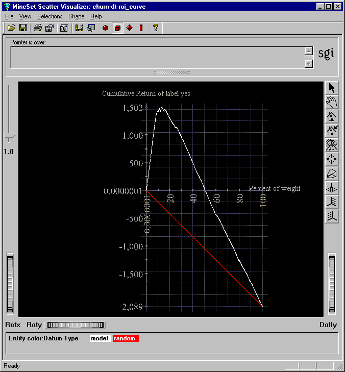
The ROI curve bears a marked resemblance to a lift curve. The horizontal line across the middle represents zero profit and loss. The red line represents the expected performance if you were to take a random sample of the population and send them mail. You expect a loss if you mail to everyone, because of the cost of mailing. However, there is a point of optimum return on investment, represented by the apex of the curve, at 1448, or 15.2 percent of the population.
Take care when filling out a Loss Matrix for use with an ROI curve. The column under a certain predicted label determines the resulting ROI curve for that label value. If you were to fill out a Loss Matrix for the churn dataset using the label churn, the entries in this column need to represent the expected gain or loss for taking the action associated with that label value, on all of the possible classes. For example, the entry under the column “prediction yes” in churn, under the row “actual value no,” may contain the value 2 to indicate that the cost of mailing a brochure (the action associated with “yes”) to someone who was not going to churn is 2 dollars. On the other hand, the entry under the column yes, row yes, may have a value of -10 to indicate that a customer was prevented from churning, saving the company 10 dollars over the cost of the mailing. These costs can be difficult to estimate, and small variations may significantly affect the position of the apex in the resulting ROI curve.
For further details, see the MineSet Enterprise Edition Reference Guide and check the MineSet website at http://mineset.sgi.com for the latest updates.