The previous chapter described how to use NetLook for an overall view of current network traffic. This chapter explains how to use NetGraph to monitor network traffic over a period of time. NetGraph's real-time strip charts delineate network usage and allow you to graph specific types of traffic such as the number of packets or the number of bytes per second. Filters can be used to restrict the graphs to the traffic of interest to you. An alarm mechanism warns when a graphed value exceeds a threshold you specify, and a history feature lets you play back previously recorded network data.
NetGraph's charts help you determine network overloading and traffic congestion. Use the information in the graphs when you want to expand or divide your network or determine where to place bridges, routers, and gateways on your network. For example, if NetLook displays intense traffic between two nodes, you can use NetGraph to graph how much traffic comes from or goes to each node, the percentage of total network traffic transmitted by each node, the times when traffic is the most intense, and so forth.
Developers of distributed applications can use NetGraph to look at the traffic rates between servers and clients and between multiple servers in applications that have them.
This chapter explains how to:
start NetGraph
use the NetGraph main window to display graphs of traffic volumes
use the NetGraph control panels to specify the type of traffic you want to view and configure the display of traffic
collect traffic information and play it back in NetGraph later
In addition, a variety of NetGraph examples are provided. For complete information on NetGraph command line options and resources, see the netgraph(1M) manual page in Appendix F, “NetVisualyzer Manual Pages.” Additional information about the NetGraph configuration file is provided in Appendix D, “Configuration File Formats.”
 | Note: You must have authorization to use NetGraph. See “Authorizing NetVisualyzer Users for Snooping” in Chapter 1 and Appendix B, “Authorization Reference,” for details. |
To start NetGraph, double-click the netgraph icon in the netvis directory view or enter:
netgraph |
The default NetGraph main window appears as shown in Figure 4-1.

When NetGraph starts, it uses a configuration file to determine the types of graphs to display. By default, NetGraph looks for .netgraphrc in your home directory. If this file does not exist, NetGraph displays a Warning window and displays the default graph in the NetGraph main window.
You can specify a configuration file on the NetGraph command line with the –u option or in the NetGraph resources file with the NetGraph*controlsFile resource.
In its default configuration, NetGraph shows a strip chart of total network traffic as measured in packets per second and displays a scrolling time legend below the graph that shows the time of day. You can add, delete, and edit graphs by using the NetGraph Edit menu.
For each protocol that NetGraph understands, it can produce a graph that shows one of the following:
packets or bytes per second
percentage of total packets or total bytes
percentage of Ethernet or FDDI capacity
percentage of a given number of packets or bytes per second
Figure 4-2 shows an example of a NetGraph main window with several graphs.
The NetGraph main window title bar includes “–i” and the interface it is snooping on. The interface is in the same format as the argument to the –i command line option.
Above each graph, two lines list the filter being used and how the traffic is being measured. For example, in Figure 4-2 the filter for the bottom graph is nfs and the traffic is measured in packets per second. Above the graph on the right side, the maximum (highest) value attained for the graph since it started and the current value of the graphed quantity are displayed.
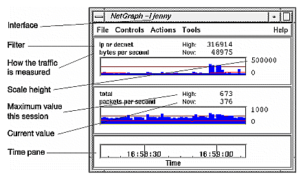
Horizontal scale lines on the graphs help you visualize values. NetGraph's minimum-sized window shows just one scale line. However, if you increase the window size, up to 4 scale lines appear to delineate 5 vertical sections. Labels for the vertical scale of the graph appear to the right of each graph.
A Time pane appears at the bottom of the NetGraph window. By default, the time type is Scrolling. It shows the absolute (real) time of day.
To select a graph, click the left mouse button in its pane. The pane background turns yellow.
NetGraph provides two control panels, Edit and Parameters, for use in setting up what NetGraph monitors and how it is displayed.
To bring up a control panel, select it from the Controls menu. The control panel is automatically placed at the location specified in a .netgraphrc file if one is being used, or in a default location otherwise.
Each of the control panels is discussed in a section below.
Use the Edit control panel to specify a filter, how the traffic should be measured, graph style, graph color, and alarms for a single graph.
To edit a graph, select the graph by clicking on it in the NetGraph main window. The values in the Edit control panel are updated to match the current values of the selected graph. An example is shown in Figure 4-3. Each section of the control panel is discussed below.
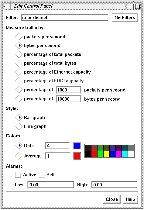
Perhaps you want to capture only certain network packets, such as packets destined for a particular node or packets of a particular protocol. To do this, use the Filter entry field shown in Figure 4-4 to capture only packets that are of interest to you.

Type the filter you want to use in the entry field and press <Enter> or use NetFilters. When you click the NetFilters button, the NetFilters main window appears. When you select a filter in NetFilters by double-clicking on it, it appears in the Filter entry field and the selected graph is automatically changed. Using NetFilters is described in Chapter 2, “NetFilters.”
The NetGraph default is to monitor the total network traffic. The NetGraph-specific filter total is used to indicate this.
To specify how the traffic is to be measured, select the Measure traffic radio button shown in Figure 4-5 that specifies the type of graph you want. The graph types are:
| packets per second |
| |
| bytes per second |
| |
| percentage of total packets |
| |
| percentage of total bytes |
| |
| percentage of Ethernet capacity |
| |
| percentage of FDDI capacity |
| |
| percentage of n packets per second |
| |
| percentage of n bytes per second |
|
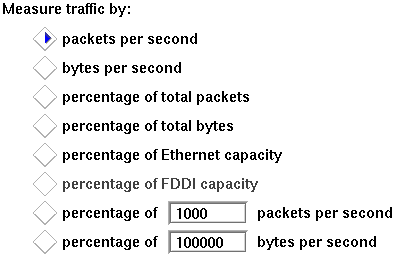
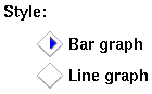
Figure 4-6 shows the Style radio buttons. Select the Bar graph radio button or the Line graph radio button to specify the graph style you want.
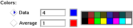
For the graph and the moving average line, the Colors entry fields and left-most color squares in Figure 4-7 display their color values and colors. The array of colors on the right show some of the possible color choices. To select a new value, first select the radio button for the color you want to change, data or moving average. You can enter a color map index in the entry field and press <Enter>, or click the left mouse button on the color square of your choice in the array of colors on the right. The color square next to the entry field is updated to reflect the new selection and the selected graph is changed.
The NetGraph alarm notifies you when a value on a graph goes above or below numbers you specify. When an alarm condition is met, NetGraph flashes pink, writes a message to a shell window or to a file you specify, and if specified emits an audible sound (a beep). The alarm is turned off by default. To set the alarm, check the “Active” check box shown in Figure 4-8. Check the “Bell” check box when you want NetGraph to beep when an alarm condition is met.

The Low and High entry fields specify the conditions when you want alarm notification. If the graph goes under the Low value or above the High value, a message appears in the window from which you invoked NetGraph. If you launched NetGraph from the netvis directory view, a message is sent to the console. When the condition is no longer met, you also receive a message. For example, the Low entry field contains 100, the High entry field contains 1000, and the filter is ip.host serendipity. Each time an alarm condition is met, messages appear on the screen:
Alarm condition met at 19:02:10:
     filter: ip.host serendipity (packets / second)
     value: 92.00 < 100.00
Alarm condition no longer met at 19:02:22:
     filter: ip.host serendipity (packets / second)
     value: 196.00 > 100.00
Alarm condition met at 19:02:34:
     filter: ip.host serendipity (packets / second)
     value: 1105.00 > 1000.00
Alarm condition no longer met at 19:03:11:
     filter: ip.host serendipity (packets / second)
     value: 996.00 < 1000.00
|
If you do not want messages to appear on the screen, you can put them in a file by starting NetGraph with the –l option. See “Writing Alarm Messages to a File” in this chapter for an example.
The Parameters control panel enables you to specify new values for the NetGraph time legend and graph scale parameters, to specify a new interface to collect data from, and to control various time intervals. Figure 4-9 shows the Parameter Control Panel window.
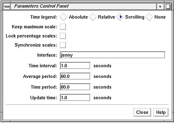
Each parameter corresponds to a NetGraph command line option; for example, a check mark in the “Keep maximum scale” check box corresponds to the –M option. See netgraph(1M) in Appendix F for the options that correspond to the choices on the Parameter Control Panel.
Figure 4-10 shows the Time legend radio buttons.

| Absolute | Show the absolute time of day of the start and end of the displayed samples. When the period of time it takes for a single sample to scroll off the graph (Time period) is set to one minute, the time legend looks similar to Figure 4-11. | |
| Relative | Show the time of the samples in the graphs relative to the current time. When the period of time it takes for a single sample to scroll off the graph (Time period) is set to one minute, the time legend looks similar to Figure 4-12. | |
| Scrolling | Display a scrolling time legend below the graphs showing the absolute time of day. When the period of time it takes for a single sample to scroll off the graph (Time period) is set to one minute, the time legend looks similar to Figure 4-13. | |
| None | Do not display a time legend.
|



Check the “Keep maximum scale” check box shown in Figure 4-14 to keep the vertical scale of all graphs at the maximum value they attain. When this check box is not checked, the graphs are rescaled down when NetGraph deems it appropriate. Rescaling provides better resolution of the graphs and occurs when the current value is greater than the maximum or when all values are low enough to decrease the scale. Maximum scale values are 10, 20, 50, 100, 200, 500, and so on. For example, if the maximum value displayed reaches 81, the graph is rescaled to 100. If the maximum value drops to 50 or below for the period of time the graph is displayed on the screen, the graph is rescaled to 50.

Check the “Lock percentage scales” check box shown in Figure 4-15 to lock the scale of all percentage graphs from 0 to 100. When this check box is not checked, (the default) percentage graphs scale like all the others.

Check the “Synchronize scales” check box shown in Figure 4-16 to synchronize rescaling of all graphs of the same type. For example, graphs displaying packets per second would all be rescaled at once. When this check box is not checked (the default), graphs rescale individually.

Leave the Interface entry field shown in Figure 4-17 blank to snoop on the local interface (the default) on the Display Station.

You can specify another interface, possibly on a remote Data Station, to snoop on using the format:
station:interface |
The default interface is understood by NetGraph, so you don't have to specify it. For example, to snoop on the default interface on a Data Station named reddog, enter:
reddog: |
Give the command netstat -i to see a list of configured interfaces. You can use any of the names in the Address column for station and the matching name in the Name column as the interface.
The NetGraph main window title bar includes “–i” and the interface you are snooping on.
Specify the sampling interval, in seconds, for all the graphs using the entry field shown in Figure 4-18. The default is to sample every second. A short time interval shows real-time network utilization levels that often appear as spikes. A longer interval shows average network utilization levels that seem smoother.

Specify the moving average calculation period of each graph using the Average period entry field shown in Figure 4-19. The default is to calculate the moving average using one minute of data. When a shorter moving average period is used, the moving average line more closely approximates the data graph. A longer average period tends to smooth out the moving average line.

Specify the period it takes for a single sample to move off the graph in seconds using the Time period entry field shown in Figure 4-20. The default is for a sample to take one minute to move off the chart. The time period cannot be less than the time interval.

If you specify a small value, the samples will scroll off the chart more quickly. If you specify a large value, the samples will display more data; this requires more memory and more time to redraw the graphs.
Set the update time in seconds using the Update time entry field shown in Figure 4-21. The default is to update every sampling interval (from the Time interval entry field). The update time determines how often graphs are redrawn. The update time cannot be less than the time interval and cannot be greater than the time period.

For example, suppose you set the time interval and update interval to .1 so NetGraph will sample and update every .1 seconds. The drawing of the graphs may not be able to keep up with real time, especially if you have a lot of graphs. However, if you specify an update rate of 1, you will get a lot of samples and still keep up with real time. This setting causes graphs to be redrawn with 10 new samples every second rather than one new sample every .1 second.
Figure 4-22 shows the Actions menu. The three choices are described in the following sections.
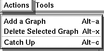
To add a graph to the NetGraph main window, select “Add a Graph” from the Actions menu. If no graph is highlighted in the NetGraph main window when you select “Add a Graph,” a new graph appears immediately above the Time pane. If a graph is selected (highlighted in yellow), the new graph appears above the selected graph. The current settings of the Edit control panel are used for the new graph. A typical sequence for adding a graph is:
Choose a location for the new graph by selecting the graph that you want the new graph above (do not select a graph if you want the new graph at the bottom).
Select “Add a Graph.”
Select the new graph by clicking on it.
Select “Edit...” from the Controls menu if the Edit control panel isn't already open.
Edit the graph as described in “Edit Control Panel” in this chapter to change the filter, graph style, alarms, and so on.
To delete a graph from the NetGraph main window, select the graph to highlight its pane in yellow, then select “Delete Selected Graph” from the Actions menu.
The display of graphs may fall behind real time, especially if you have many graphs and a small sampling interval. To catch up to real time, select “Catch up” from the Actions menu. To catch up, NetGraph will average all data it skips, so the graphs will appear level for the skipped time. NetGraph may occasionally catch up by itself if it falls very far behind real time, or in some cases when you add or delete a graph.
The NetGraph File menu lists three choices: “Save Controls,” “Save Controls As...”, and “Quit.” These choices are described below.
The “Save Controls” choice enables you to save NetGraph configuration information. It saves user interface configuration information to the user interface file you last specified with “Save Controls As...” (if any) or the file read when NetGraph started up.
By default, the file ~/.netgraphrc is read when you start NetGraph; you can specify a different user interface configuration file at startup with the –u command line option.
The “Save Controls As...” choice enables you to save NetGraph user interface configuration information to a file name of your choice. When you select “Save Controls As...”, a file prompter window appears. Use the procedure in the section “Using a File Prompter” in the Introduction to specify the file name for the configuration data.
By default, the file ~/.netgraphrc is read when you start NetGraph; you can specify a different configuration file at startup with the –u command line option.
To exit NetGraph, select “Quit” from the File menu. A NetGraph Question window appears. To save the current configuration in the file shown in the message and quit NetGraph, click the Yes button. To quit without saving configuration information, click the No button. If you want to write the information to another file or decide not to quit NetGraph, click the Cancel button.
You can collect NetGraph data, put it in a history file, and review the data at a later time.
To collect data and write it to a history file, give the NetGraph command with the –o option:
netgraph –o file |
where file is the name of the file in which to put the data. If the file exists, and is currently being used by another NetGraph, you cannot write history data to it; if the file exists and is not in use by another NetGraph, it will be overwritten with the new data.
For example, to save the date to a file named netgraph_hist, type:
netgraph –o netgraph_hist |
The NetGraph window appears on the screen as described previously in this chapter. NetGraph data is written to the file you specified. To stop data collection, just quit NetGraph.
An option that can be used only when you give the –o option is the –O (capital O) option. When you give this option, traffic data is printed to standard output as well as the history file.
To play back the data, give the command:
netgraph –i file |
For example, to play back the data from netgraph_hist, enter:
netgraph –i netgraph_hist
The title bar of the NetGraph main window displays the name of the file you specified on the command line (for example, netgraph_hist). The graph specifications and options are read from the history file and the graphs automatically replay the data that was previously captured. The bars/lines scroll from right to left, and the time legend is updated.
An additional pane with history controls appears at the bottom of the window. Figure 4-23 shows the history controls.
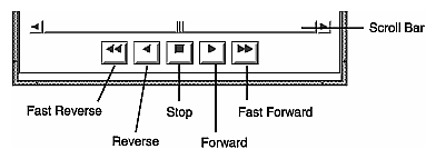
While you are playing back a history file, not all features of NetGraph are available since only the stored data is available. However, many options on the Edit and Parameter control panels can be used. These control panels appear in abbreviated versions when you are playing back a history file.
This section includes several examples of NetGraph use:
using some simple filters
monitoring several network segments from a single Display Station
using NetGraph information collected over time
monitoring internetwork traffic
writing alarm messages to a file
You can use any valid filter expression in the Filter entry field on the Edit control panel. For example, you may want to capture only User Datagram Protocol (UDP) packets on the network. In this case, the filter consists of a simple one-word expression: udp. This expression is a macro that expands to ip.udp. (To see the macro definition, give the command netsnoop -L ether.)
To capture all IP packets between two nodes named gary and indiana, enter this expression in the Filter entry field:
ip.between(gary,indiana) |
To create a filter expression, use logical operators to combine protocols, functions, macros, and constants as described in Chapter 10, “Creating and Using Filters.” Some examples of filters are:
| ip | Internet Protocol traffic | |
| tcp or nfs | TCP or NFS traffic | |
| dst=8:0:69:1:4:93 |
| |
| udp and ip.src=indiana |
|
This section describes how to monitor three network segments from a central Display Station. You can do this provided a Data Station is connected to each network segment and you have authorization to snoop from the respective Data Stations. For information on authorization, see “Authorizing NetVisualyzer Users for Snooping” in Chapter 1.
Suppose you want to run three NetGraph sessions from the central Display Station—one that snoops locally on the Display Station and two other sessions that snoop on the two remote Data Stations. You also want to gather different information from each network. To do this, create a different configuration file for each network, and then create a script that runs the files.
For example, suppose the networks are named building1-net, building2-net, and building3-net. The Display and Data Stations are named netvis-station1, netvis-station2, and netvis-station3. Follow the steps below to monitor the three network segments.
Use NetGraph to create three configuration files to capture data from each Data Station. Just use the Edit and Parameters control panels to specify how you want the graphs set up. Then save the first NetGraph configuration (for example save it as .netgraphrc1) but do not quit NetGraph. Next edit the graphs for the second network and save the configuration as a new file name, .netgraphrc2, for example. If you wish, you can use an editor such as vi(1) to add comments to each file, for example, # configuration for building1-net. The files look like this:
# configuration for building1-net
option -i netvis-station1 -t .5
total bytes
nfs packets
“ip.between(node4, node5)” line
# configuration for building2-net
option -i netvis-station2
total bytes
nfs packets
# configuration for building3-net
option -i netvis-station3 -t 2
total bytes
“nfs or udp” %packets line
Each file has the NetGraph options and graph specifications for the NetGraph session that will snoop on the respective Data Station. The key item in each file is the –i option that specifies the Data Station on which to snoop.
Create a shell script to run the three NetGraph sessions, each with the appropriate configuration file. For example, name the file netgraph_3; it looks like this:
netgraph –u .netgraphrc1
netgraph –u .netgraphrc2
netgraph –u .netgraphrc3
Make sure this file is executable by typing the following at a shell prompt:
chmod +x netgraph_3
Now start three sessions of NetGraph, each snooping on different network segments, just by typing:
netgraph_3
That's all there is to it. You can monitor as many networks as you want providing each network has a Data Station connected to it.
Since NetGraph shows network traffic over a period of time, it is useful in seeing how various types of traffic vary throughout the day or week.
Measuring traffic as packets per second tells you how the CPU resources in the network are being interrupted and used for protocol passing. This is often the most resource-consuming task in a network environment. For example, if you are using an NFS server for file-sharing among an increasing number of clients, you can use NetGraph to monitor the load on the NFS server and determine when subnetting and additional servers are needed.
Monitoring traffic as %ether or %fddi shows total bandwidth use. For example, if utilization is consistently above 30% for Ethernet, consider dividing the network.
Observing packet traffic between interconnected networks provides information for determining packet-routing requirements for bridges, routers, and gateways. Configuring these internetworking devices with adequate packet-processing capacity eliminates traffic congestion, improves network response, and enhances internetwork communications.
Suppose the network is divided into smaller networks and at times exhibits performance degradation. You suspect the interconnecting routers or gateways may have inadequate packet-processing capacities.
Use NetGraph to monitor the traffic going through a specific routing device. Figure 4-24 shows a router with two interfaces: router1 with physical address 2:26:2:3:2:4 and router2 with physical address 2:26:2:3:2:5.
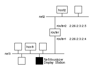
Use a filter expression at the command line to request that NetGraph capture and display only Ethernet packets with address 2:26:2:3:2:4 as either the source or the destination node. In other words, capture only internetwork traffic through router1.
Enter this filter in the Filter entry field of the Edit control panel:
host 2:26:2:3:2:4 |
NetGraph displays a graph of varying traffic load on router1, the routing device between net1 and net2. This measure (in packets per second) also represents the number of internetwork packets between the two networks that router must be able to process per second. If router1's traffic load exceeds its specified packet processing capacity, router1 may be a bottleneck in passing information between the two networks.
When a router is the bottleneck in internetwork traffic, slower network response occurs. Imagine node1 in net1 trying to send a packet to node2 in net2 (see Figure 4-24) and the packet fails to enter the queue at router1 to be processed. node1 has to send the same packet again, thus consuming twice as much of net1's bandwidth.
NetGraph, like other NetVisualyzer tools, offers filtering capabilities for isolating traffic for analysis. For example, if an NFS workgroup is part of a multivendor network, you may want to monitor only varying NFS traffic loads in the network. Enter this filter in the Filter entry field of the Edit control panel:
nfs |
This filter causes only NFS traffic to be displayed. When the traffic load is measured in packets per second, the NetGraph graph shows the interrupt load on the NFS server for processing of file-sharing services. Also, the load measure in bytes per second reflects the amount of data flow between an NFS server and its clients.
As different NFS servers have different interrupt and transfer-throughput capabilities, it's up to you to decide when to divide an NFS workgroup and add servers. NetGraph helps you to predict how different NFS servers will behave in similar configurations.
When you check the “Alarm” check box in the Edit control panels for a graph, alarm messages are written to your console or the shell window from where you started NetGraph. To write these messages to a file instead, start NetGraph with the –l option:
netgraph -l file |
where file specifies the name of the message file. Messages are appended to the end of this file.