Volumetric data produced by acquisition devices, such as computer tomography (CT) or magnetic resonance imaging (MRI) devices used in medical imaging, is usually regularly spaced data where the space between adjacent sample points remains constant throughout the volume data. In certain applications, however, the sample points can be at arbitrary positions in world space. These kinds of irregular grids are commonly found in computational fluid dynamics (CFD) applications. For example, a CFD application can use these sample points to represent the space around an aircraft and then use computer simulations to compute the various fluid parameters, such as pressure and energy, at these sample points. Using irregular grids allows the grid to be more densely sampled at special regions of interest and sparsely sampled at other locations. This approach provides more accurate simulations for critical parts of the object under consideration—the nose of the aircraft, for example. Figure 7-1 shows the wireframe model of such a grid, which models the flow around a wing. Note how the data is highly sampled at the tip of the wing and sparsely so at other locations.
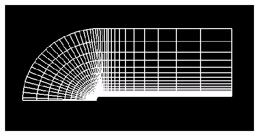
Volume visualization of such datasets is critical in detecting the specific features in these datasets since conventional techniques like the use of isosurfaces and particle tracing are not able to reveal certain 3D structures in the data. Various techniques can be used to volume render such datasets. A commonly used approach is to resample the irregular grid to a conventional volume dataset using interpolation techniques. Such a process can be computationally expensive and, also, using a regular sampling can result in loss of critical details at areas of high density.
This chapter describes how OpenGL Volumizer renders irregular grids in the following sections:
The Projected Tetrahedra Render Action ( PTRenderAction) provides a new render action for volume rendering irregular grids. The render action uses the following steps to render the grid:
Tessellate the input volumetric geometry into a tetrahedral representation.
Sort the tetrahedra in back-to-front visibility order using a fast sorting algorithm.
Render the grid by projecting each tetrahedron to the screen in the sorted order.
Apply color and opacity to the rendered geometry using the shading parameters (lookup tables, and the like).
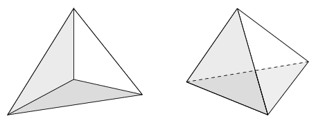
The main difference between the algorithm used by the Texture Mapping Render Action (TMRenderAction) and PTRenderAction is in the polygonization step. Polygonization is the process of approximating the volumetric geometry (tetrahedra) using polygonal geometry (triangles) to allow direct rendering using OpenGL hardware. TMRenderAction approximates each rendered tetrahedron by computing proxy geometry by intersecting with viewport-aligned slices. PTRenderAction projects each tetrahedron into screen space using a footprint evaluation technique.
Figure 7-2 shows two different approximations of a tetrahedron projected into screen space. The first approximation uses three triangles and the second one uses four triangles.
Both PTRenderAction and TMRenderAction are derived from the base class vzRenderAction. Both provide the manage(), unmanage(), and draw() methods for resource management and rendering of volumetric shapes.
The following code sample creates a PTRenderAction and uses it to manage and render a shape node:
vzPTRenderAction *renderer = new vzPTRenderAction; renderer->manage(shape); renderer->beginDraw(0); renderer->draw(shape); renderer->endDraw(); |
The render order of a shape is determined by the invocation of its draw method. Consequently, the application must sort the multiple shapes being rendered in the desired visibility order. The render action provides all the data management internally using a lazy evaluation technique.
The PTRenderAction supports multiple sorting algorithms to sort the tetrahedral grids before rendering. Choose a sorting algorithm that matches the input grid that is being rendered. PTRenderAction supports the following sorting modes:
VZ_CONCAVE
VZ_CONVEX
VZ_NO_SORT
The default mode is VZ_CONCAVE, which uses a linear order sorting algorithm for fast sorting of concave meshes. The sorting provides good visual quality but does not guarantee the correct order for certain boundary anomalies.
Use the VZ_CONVEX flag to provide accurate sorting if the grid is known to be convex. Use the VZ_NO_SORT flag to disable visibility sorting, in which case the volumetric geometry will be rendered in the order specified by vzIndexArray. The following code sample selects the concave sorting algorithm:
renderer->setSorter(VZ_CONCAVE); |
Note that the sorting and tetrahedral projection steps are computed entirely in software and, consequently, constitute the bulk of the rendering time. Due to lack of hardware support, the rendering is usually not as interactive (between software and hardware) as in the case of 3D textures, for which there is support in the graphics hardware. On Silicon Graphics Prism systems, the projection algorithm can be implemented using the programmable vertex and fragment engines. This process is transparent to the application.
For certain datasets, it is useful to use other rendering techniques in conjunction with the projected tetrahedra algorithm to visualize the dataset. PTRenderAction also supports the following two rendering methods:
| drawBoundary() | Renders the grid boundary. | |
| drawCells() | Renders cells. |
The rendered primitives can be controlled by setting the OpenGL state with glPolygonMode() to the desired primitive—namely, GL_FILL, GL_LINE, or GL_POINT (see the glPolygonMode man page). Figure 7-1 was generated using the following code:
glPolygonMode(GL_FRONT_AND_BACK, GL_LINE); renderer->drawCells(shape); |
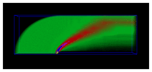
When using regular volumetric data, the volumetric geometry simply provides a region of interest for the 3D volume. Consequently, this geometry usually is a block geometry. The irregular grids produced by CFD applications typically tend to be of two kinds: structured hexahedral grids and unstructured tetrahedral grids. Structured hexahedral grids (also referred to as curvilinear grids) can be thought of as a “warped” and “scaled” regular volume because each vertex in the grid can be indexed using a 3-tuple, just like a regular volume. Therefore, the ordering of the vertices in the grid is implicit, and each set of eight neighboring vertices represent a hexahedron. The Blunt Fin dataset, shown in Figure 7-3, is an example of a structured hexahedral grid with dimensions of 40x32x32. An unstructured tetrahedral grid, however, can have vertices at arbitrary locations and, therefore, needs to be indexed linearly using a vzIndexArray (see “Shape-Related Classes” in Chapter 3). An application can use its own volumetric geometry class as long as it overrides the virtual tessellate method to create a tetrahedral representation of the geometry.
The Blunt Fin dataset, shown in Figure 7-3, represents airflow over a flat plate with a blunt fin rising from the plate. The free stream flow direction is parallel to the plate and to the flat part of the fin, entirely in the X axis direction. The flow is assumed to be symmetrical about a plane through the center of the fin. Consequently, only one half of the “real” geometry is present and used in the computation.
PTRenderAction supports only one shader, vzPTLUTShader. The vzPTLUTShader volume renders the data using color and opacity, which are specified using the shader parameter vzParameterLookupTable. The following are the required parameters for vzPTLUTShader:
The following sections describe the shader parameters vzParameterVertexData and vzParameterLookupTable .
Each vertex in the output grid is associated with a set of floating point values which correspond to the computed data values at that vertex. The application can specify these data values using the class vzParameterVertexData, which allows storing a set of floating point values for each vertex in the grid. For example, Plot3D solution files store five values per vertex—namely, pressure, momentum (3-tuple), and energy. This can be represented using a vzParameterVertexData as follows:
// Five values per vertex
vzParameterVertexData *vertexData =
    new vzParameterVertexData(5, numVertices, dataPtr);
|
The data values need to be interleaved in the form of n-tuples, similar to the vertex coordinates in the vzVertexArray class.
The lookup_table value specifies the transfer function used to map the per-vertex data values to color and opacity values. Because the values in vzParameterVertexData can be arbitrary floating point values, the mapping is done linearly between the minimum and maximum data values for the whole grid. For example, if the range of data values is [–0.56..1.25], then the first entry in the table would correspond to –0.56 and the last to 1.25. The indices for the intermediate values can be computed by linearly interpolating between the range. Figure 7-3 shows a snapshot of the Blunt Fin dataset rendered using vzPTLUTShader.
The vzPTLUTShader uses a simple approximation for the volume density model to compute the volume rendering integral when rendering the projected tetrahedra. The transfer function for the volume renderer is implemented using a 2D texture map. This texture map is indexed using the scalar value at the rendered vertex as the “s” coordinate and the cell thickness as the `t' coordinate.
For more details on transfer functions, see “The vzParameterLookupTable Parameter” in Chapter 4.
Plot3D is a commonly used data format for storing CFD datasets. OpenGL Volumizer includes a new loader library to load Plot3D data grid and solution files into OpenGL Volumizer geometry and vertex data objects, respectively. The loader library, libvzplot3d.so, is installed in /usr/lib* and the corresponding header file is installed under VZROOT/src/lib/loaders/Plot3dLoader.h. The loader supports reading in both single-zone and multizone grids. The grids can be structured as well as unstructured and with or without an IBLANK array. The data files are assumed to be in binary format and all the floating-point data are assumed to be in 32-bit IEEE format, SGI endian. The following code loads a Plot3D grid and the corresponding solution file into an OpenGL Volumizer application:
// Create the Plot3d loader. Use the grid and solution (or scalar) // field file names Plot3dLoader *loader = Plot3dLoader::open(gridFileName, solnFileName); // Load the Plot3d grid vzGeometry *geometry = loader->loadGrid(); // Load the Plot3d solution data vzParameterVertexData *vertexData = loader->loadSolution(); |