This chapter discusses the components and capabilities of the Rules Visualizer. It first provides an overview of this data mining and visualization tool, then it explains this tool's functionality when working with the
main window
external controls
pulldown menus
Finally, it lists and describes the provided sample files for these tools.
The Rules Visualizer gives you the power to mine data by constructing, verifying, and graphically representing models of patterns in large databases. These patterns are expressed via association rules, which indicate the frequency of items occurring together in a database.
Discovering and graphically displaying association rules can be relevant to many enterprises, including supermarket inventory planning, shelf planning, and attached mailing in direct marketing.
The tool execution scenario described in Chapter 1 of this document (see Figure 1-1) is slightly modified for the Rules Visualizer. First, the “raw” data in your database must be converted into a specially formatted file that can be processed by the association rules generator part of the Rules Visualizer. When the association rules generator has processed this file, the results can be displayed by the rules visualizer part of this tool.
Thus, the Rules Visualizer consists of three operations:
Data conversion. The association data converter processes a “raw” data file and creates a file usable by the association rules generator.
Association rules generation. The data file created by the association data converter is processed by the association rules generator, which creates a file usable by the rules visualizer.
Rules visualization. This operation displays the generated association rules.
In addition to the input data and rules file requirements, each operation requires a configuration file that specifies operational parameters.
The sequence of actions by the user, at the user's workstation, and at the host server is shown schematically in Figure 9-1. The phases indicated at the right of the illustration correlate to the operations listed above.

The association data converter takes a “raw” data file, such as one resulting from a database query, and creates a binary data file in the format used by the association rules generator. The internal format of this generated file allows optimum processing by the rules generator. The data converter also accepts input from flat files as well as databases.
One example of applying the association rules generator is to obtain “market basket” data for customer buying patterns. Here, “market basket” is the set of items bought by each customer on a single visit to a store. An example rule in this context might be: “80% of the people that buy diapers buy baby powder.” This percentage is known as the predictability of the rule.
In the example, “diapers” is the item on the left-hand side (LHS) of the rule, and “baby powder” is the item on the right-hand side (RHS) of the rule.
Some applications of these rules are as follows:
If “Fizzy Pop” appears on the RHS, the LHS can help us determine what the store should do to boost sales of this beverage.
If “Bagels” appears on the LHS, the RHS can help us determine what products might be affected if the store no longer sells bagels.
The association rules generator part of this tool processes an input file, then generates an output file consisting of the rules. If X and Y are items in a record, then a rule such as
X fi Y
indicates that whenever X occurs in a record, expect Y to occur with some frequency.
The strength of the association is quantified by three numbers. The first number, the predictability of the rule, quantifies how often X and Y occur together as a fraction of the number of records in which X occurs. For example, if the predictability is 50%, X and Y occur together in 50% of the records in which X occurs. Thus, knowing that X occurs in a record, expect that 50% of the time Y occurs in that record.
The second number, the prevalence of the rule, quantifies how often X and Y occur together in the file as a fraction of the total number of records. For example, if the prevalence is 1%, X and Y occur together in 1% of the total number of records.
You can specify a minimum prevalence threshold for the generated rules. The default minimum prevalence threshold is 1%. The lower the minimum prevalence, the more rules are generated, and the slower the performance of the tool might be. You can also specify a minimum predictability threshold for the generated rules. The minimum predictability threshold default is 50%.
Rules that meet a minimum prevalence threshold are important for two reasons:
A rule might have business value only if a reasonably significant fraction of records support the rule. For example, if everyone who buys caviar also buys vodka, the rule Caviar ⇒Vodka has 100% predictability. However, if only a handful of people buy caviar, the rule might be of limited value to the retailer.
A rule might not be statistically significant if a very small number of records support the rule. The rule might be due to chance, and it would not be prudent to make decisions based on such a rule.
The third number is expected predictability. The expected predictability is the frequency of occurrence of the RHS items. So the difference between expected predictability and predictability is a measure of the change in predictive power due to the presence of the LHS rule. Expected predictability gives an indication of what the predictability would be if there were no relationship between the items.
The Association Rules generator does not report rules in which the predictability is less than the expected predictability. In other words, a rule such as A->B is not reported if the frequency of A and B occurring together is less than the frequency of B alone.
 | Note: Given just Y and a rule of the form X ⇒ Y, nothing is known about X. Rules specify implications only from the LHS to the RHS. |
Table 9-1 summarizes the three numbers that quantify the strength of each association rule.
Table 9-1. Association Rules Components
Measure | Description |
|---|---|
Prevalence | Frequency of LHS and RHS occurring together. |
Predictability | Fraction of RHS out of all items with LHS, or the prevalence divided by the frequency of occurrence of LHS items. |
Expected Predictability | Frequency of occurrence of RHS items. |
The rules generator also works on hierarchical data, which includes a component that relates (or maps) data to new data at varying degrees of generality. The ability to handle hierarchical data allows rules to be generated at the desired level of generality.
For example, consider the hierarchy shown in Table 9-2. This hierarchical information, in addition to the “market basket” data that lists the products purchased in each record, allows rules to be generated at four levels. In contrast to rules learned at the lowest level, which relate specific products to each other, a rule at the highest level might be “Milk implies Bread.”
Table 9-2. Example of Hierarchical Levels
Level | Example |
|---|---|
Product Group | Milk |
Category | Non-Refrigerated Milk |
Brand | Lucerne® |
Product ID (UPC/SKU Code) | 1 pint can of Premium Condensed Milk |
The rules visualization part lets you graphically display and explore the generated association rules. The rules are presented on a grid landscape, with left-hand side (LHS) items on one axis, and right-hand side (RHS) items on the other. As shown in Figure 9-2, attributes of a rule are displayed at the junction of its LHS and RHS item. The display can include bars, disks, and labels.

If the displayed view is too small, item labels do not appear on the side of the axes. You can zoom in on the view until the item labels appear (see the Dolly description in “Thumbwheels” in Chapter 6).
A legend indicating the mapping between displayed attributes (such as bar heights and colors) and the values associated with the underlying rules (such as predictability and prevalence) can be displayed at the bottom of the main window.
The Tool Manager interface for associations allows you to run the Rule Visualizer without running associations, by using the Visual Tools menu from Tool Manager's main window.
Each of the Rules Visualizer's three components has its own file requirements. These are detailed in the following subsections.
A “raw” data file that results from extracting raw data from a source (such as a relational database). This file is processed by the association data converter to produce the internal binary data file used by the association rules generator.
A format file that specifies the format of the data file. If the internal binary data file (see next subsection) is created via the Tool Manager, this format file is created automatically. If the internal binary data file is created via the command line, this format file must be created manually (see Appendix F, “Creating Data and Configuration Files for the Rules Visualizer”).
An internal binary data file, which results from running the association data converter on your original data.
If you have hierarchical data, the association rules generator also requires the following two files:
A mapping file, which specifies the mapping between hierarchical levels.
A description file, which specifies a string description for each item at a specific hierarchical level.
A rules file that results from running the association rules generator.
A .ruleviz configuration file that specifies parameters used by the rules visualizer program (such as mapping colors to prevalence values) when displaying the generated rules. This file is easily created using the Tool Manager (see Chapter 3). You also can use an editor (such as jot, vi, or Emacs) to produce this file (see Appendix F, “Creating Data and Configuration Files for the Rules Visualizer”).
The Rules Visualizer has three components. The following subsections describe the procedure for starting each one.
There are two ways to start the association data converter part of the Rules Visualizer:
Use the Tool Manager to configure and start the data converter. (See Chapter 3 first for details on most of the Tool Manager's functionality, which is common to all MineSet tools; see below for details about using the Tool Manager in conjunction with the data converter.)
Enter the following command at the UNIX shell command-line prompt:
assoccvt parameters
The parameters are described in Appendix F, “Creating Data and Configuration Files for the Rules Visualizer.”
There are two ways to start the association rules generator part of the Rules Visualizer:
Use the Tool Manager to configure and start the association rules generator. (See Chapter 3 first for details on most of the Tool Manager's functionality, which is common to all MineSet tools; see below for details about using the Tool Manager in conjunction with the association rules generator.)
If the data with which you are working is non-hierarchical, enter this command at the UNIX shell command line prompt:
assocgen parameters
If your data is hierarchical, enter this command at the UNIX shell command-line prompt:
mapassocgen parameters
The parameters for both instances are described in Appendix F, “Creating Data and Configuration Files for the Rules Visualizer.”
There are five ways to start the rules visualization part of this tool:
Use the Tool Manager to configure and start the Rules Visualizer. (See Chapter 3 first for details on most of the Tool Manager's functionality, which is common to all MineSet tools; see below for details about using the Tool Manager in conjunction with the Rules Visualizer.)
Double-click the Rules Visualizer icon, which is in the MineSet page of the icon catalog. The icon is labeled ruleviz. Since no configuration file is specified, the start-up screen requires you to select one by using File > Open.
If you know what configuration file you want to use, double-click the icon for that configuration file. This starts the Rules Visualizer and automatically loads the configuration file you specified. This only works if the configuration filename ends in .ruleviz (which is always the case for configuration files created for the Rules Visualizer via the Tool Manager).
Drag the configuration file icon onto the Rules Visualizer icon. This starts the Rules Visualizer and automatically loads the configuration file you specified. This works even if the configuration filename does not end in .ruleviz.
Enter this command at the UNIX shell command-line prompt:
ruleviz [ configFilename ]
When starting the rules visualization part of this tool, you must specify the configuration file, not the data or rules file.
This section describes how the components of the Rules Visualizer can be configured using the Tool Manager. Although the Tool Manager greatly simplifies the task of configuring the Rules Visualizer, you can construct a configuration file for this tool using an editor (see Appendix F, “Creating Data and Configuration Files for the Rules Visualizer”).
Note that the steps required to connect to a data source are described in Chapter 3.
The sections below follow the configuration and invocation of the Rules Visualizer components in the conventional order:
creating a file for the association rules generator
generating rules
displaying rules
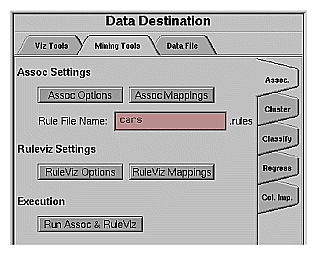
To show how to set up associations, the following example uses the cars database table. Assume that you want to find out if there is an association between miles per gallon, horsepower, and the year the car was built. For example, did mileage improve over time? Did engines become less powerful? The following steps (and Figure 9-3) show you how to set up the associations and map table columns to the data you want to study.
Connect to a MineSet server. Refer to Chapter 2, “Setting Up MineSet,”if you need help.
Open a data source.
(Optional step) In the Data Transformations tab you can choose the transformations you want do on the data before you give it to the associations engine. One recommended transformation is to create bins for numeric data. (The binning operation and the options available for it are described in detail in Chapter 3.) This leads to more “meaningful” rules from the association engine. For example, instead of using discrete values for the weightlbs attribute in the “cars” table such as 3504, 3693, 3436, 3433, and so on, it may be more meaningful to give weightlbs_bin value ranges such as 1600-2500, 2501-3500, and so on.
For this example, click on the Bin Columns button, and select all the columns in the Bin Column window for binning.
Note: If you run associations without binning any of the numerical columns (ints, floats, doubles) you get the warning message
Running associations on unbinned non-categorical data. Binning is recommended for producing more useful results.Choose the Mining Tools tab from the Data Destination tab.
Choose the Assoc. tab (abbreviation for Associations) from the Mining Tools tab.
After selecting a data source, you can run the Association Rules generator. You can choose options for this by clicking on the Assoc Options button. This causes the dialog box in Figure 9-4 to be displayed.
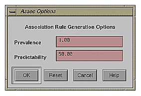
Prevalence—lets you specify the minimum prevalence threshold as a percentage of the total number of records. Rules with a prevalence below this value are not generated. The default is 1%. The possible values are 0–100.
Predictability—lets you specify the minimum predictability threshold for rules. Rules with a predictability below this value are not generated. The default is 50%. The possible values are 0–100.
Once you have made your association rule options selections, click the OK button. This returns you to the Tool Manager startup screen.

The database in the Current Columns text panel can contain multiple table columns. By mapping specific columns to association rules, the association rules generator can find the association between any possible pair of those items.
Click on Assoc. Mappings button to open the Mapping Columns to Assoc Items dialog box.
The Mapping Columns to Assoc Items window shows two panels:
Columns shows the columns in the data
Items shows the mapping between columns in the data and items
The Map All button on this window can be used to map all the attributes in the data source to items for the associations engine. The Clear All and Clear Selected buttons can be used to clear/change the mapping between columns and items.
The default behavior is to map all columns to items. Therefore, if you omit this step or if you open this window, you find all columns mapped. For this example, click OK.
Clicking on the Ruleviz Options button causes a new dialog box to be displayed (Figure 9-6). This lets you change some of the Rules Visualizer options from their default values.

This dialog box has two panels: the top one lets you set options for bars and disks; the bottom one lets you specify options for items, the grid, and labels.
Items in the top panel are listed below:
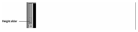
Height button—lets you specify whether the bars and disk heights are to be normalized so that the tallest bar equals the height field value (Max Height), or whether they are to be scaled by the height field value (Scale Height).
Height field—lets you enter the maximum or scale value for bar and disk heights.
Hide Distance—lets you specify the distance at which disks are not graphically represented. Smaller numbers in this field specify a shorter distance; this means fewer disks are shown and performance is greater. Larger numbers indicate a greater distance; this means disks further away remain visible.
Legends—lets you enter a text string that appears as mapping information displayed at the bottom of the main Rules Visualizer window. This is information about mapping between display entities and data values (for example, bar height corresponds to predictability values).
Color list—lets you add or edit a color. To add a color to the list, click the + button. To edit a color, click the color. See “Choosing Colors” and “Using the Color Browser” in Chapter 3 for a more detailed explanation of how to choose and change colors.
Mapping—lets you specify whether the color change that is shown in the graphic display is Continuous or Discrete. If you choose Continuous, the color values (of the bars or disks) shift gradually between the colors entered in the Color list field as a function of the values that are mapped to those colors in the Color list field.
If you
used the Color Browser to apply red and green (for bars and/or disks)
selected Discreet for the Mapping
entered the values 0 100
then the display shows all bars and/or disks with values of less than 50 in red, and all those with values greater than or equal to 50 in green.
If you
used the Color Browser to apply red and green (for bars and/or disks)
selected Continuous for the Mapping
entered the values 0 100
then the display shows all bars and/or disks with values less than or equal to 0 as completely red, those as greater than or equal to 100 as completely green, and those between 0 and 100 as shadings from red to green.
If no mapping and values are specified, a continuous mapping is used, and values are generated automatically from the minimum value to the maximum value in the data.
Items in the bottom panel are as follows:
Items On and Grids On checkbox buttons let you determine whether items (the names on the side of the grid) are displayed or hidden.
Size (for Items, Grid, and Bar Labels) lets you specify the size for items, the grid, and bar labels. If you mapped a column value to bar labels in the Requirements panel of the Tool Manager startup screen, you can specify a size for those labels.
Color (for Left-Hand Items, Right-Hand Items, Grid, and Bar Labels) lets you specify the color for LHS and RHS items, the grid, and bar labels. If you mapped a column value to bar labels in the Requirements panel of the Tool Manager startup screen, you can specify a size for those labels.
Hide Distance lets you specify the distance at which the LHS items, RHS items, grid, or labels become invisible. Smaller distances might improve performance, but the objects disappear more quickly. The higher the number, the greater the distance at which labels are hidden.
Message lets you specify the message displayed when the pointer is moved over an object or when an object is selected. (See Figure 9-8.) The syntax of the message string is the same as for the mapviz message string. See the Message Statement section in Appendix C, “Creating Data, Configuration, Hierarchy, and GFX Files for the Map Visualizer.”
The Rules Visualizer lets you map attributes of the rules to visual elements of the display. Clicking on the RuleViz Mappings button brings up the Ruleviz Mappings panel shown in Figure 9-7.
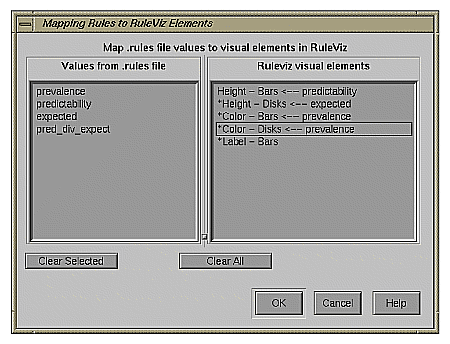
The visual elements that can be mapped are listed below, where the items with “*” are optional:
Height - Bars—lets you specify what the bar heights represent.
*Height - Disks—lets you specify what the disk heights represent.
*Color - Bars—lets you specify what the bar colors represent.
*Color - Disks—lets you specify what the disk colors represent.
*Label - Bars—lets you specify what the bar labels represent.
The default mappings are as follows:
predictability to bar heights
expected predictability to disk heights
lift to bar and disk colors
Lift is the predictability divided by the expected predictability.
The Rules Visualizer part of this tool graphically displays the data in a rules file using the specifications of a valid configuration file. For example, specifying group.ruleviz results in the image shown in Figure 9-8.
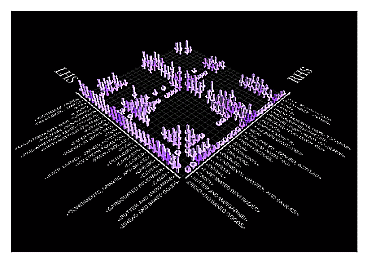
The rules are presented on a grid, initially displayed with left-hand side (LHS) items displayed on the left side of the window and right-hand side (RHS) items on the right. A rule is displayed at the junction of its LHS and RHS items. The display can include bars, disks, and labels.
When the scene is close enough, the LHS and RHS axes are labeled with the item names, unless this has been turned off in the configuration file. (To view the grid and rules at closer range, use the Dolly thumbwheel, described in the “Thumbwheels” in Chapter 6.)
You can change the labels as well as what the heights and colors of the bars and disks represent by modifying the configuration file via the Tool Manager (see Chapter 3) or using an editor to change the configuration file.
For example, in Figure 9-8, bar heights correspond to predictability values, bar colors correspond to prevalence values, and disk heights correspond to expected predictability.
The two modes of viewing are grasp and select. To toggle between these modes, press the Esc key. You also can change from one mode to the other by clicking the appropriate button: to enter select mode, left-click the arrow button (to the top right of the main window); to enter grasp mode, left-click the hand button (immediately below the arrow button, near the top right of the main window as shown in Figure 9-2).
In grasp mode the cursor appears as a hand. This mode supports panning, rotating, and scaling the scene's size in the main window.
To rotate the display, press the left mouse button and move the mouse in the direction you want to rotate. (Also see the rotating controls Rotx and Roty described in “Thumbwheels” in Chapter 6.)
To pan the display, press the middle mouse button and drag it in the direction you want the display panned.
To move the viewpoint forward, press the left and middle mouse buttons simultaneously and move the mouse downwards. To move the viewpoint backward, press the left and middle mouse buttons simultaneously and move the mouse upwards. This is equivalent to the functions provided by the Dolly thumbwheel.
In select mode, you can obtain additional information about a rule by placing the cursor over a bar. This highlights the selected bar and causes information about the rule represented by that bar to appear at the top of the main window.

The information is displayed as long as the cursor remains over the object. If you position the pointer cursor over an object and click the left mouse button, that same information appears in the Selection Window, which is above the main window, under the “Selection” label.
This Selection information remains visible until another object is selected, or until no object is selected (if you click the black background). Using the mouse, you can cut and paste this text into other applications, such as reports or databases.)
Several external controls surround the main window, including buttons and thumbwheels. (These and the rest of the buttons are the same as the other MineSet visualization tools and are described in “Buttons” in Chapter 6, and “Thumbwheels” in Chapter 6)
The Rules Visualizer has three pulldown menus, labeled File, View, and Help.
The File menu (Figure 9-11) contains six options.
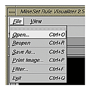
Open loads and opens a configuration file, displaying it in the main window. Previously displayed data is discarded.
Reopen reloads the current configuration file. This is useful if either the configuration file or data file has changed.
Save As... allows uyou to save the file under a different file name
Print Image... allows you to print the image from the screen
Filter....allows you to filter the data.
The Filter menu brings up a Filter panel (Figure 9-12) that lets you reduce the number of rules displayed in the main viewing area, based on one or more criteria. You can use the filter panel to fine-tune the display, emphasize specific information, or simply shrink the amount of information displayed.
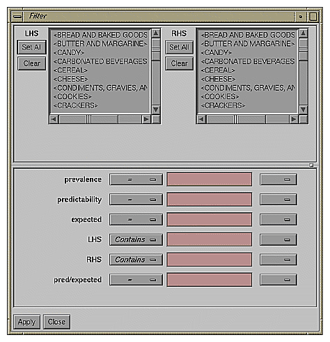
The top pane lets you filter based on string variables, such as LHS and RHS. To select all values of a variable, click Set All. To clear the current selections, click Clear. To select a value, click it. To deselect a value, click it again.
The bottom pane lets you filter based on the values of both string and numeric variables.
To filter numeric values, enter the value, and select a relational operation (=, !=, >, <, >=, <=). To filter alphanumeric values, enter the string. You can use any of three types of string comparisons:
Contains indicates that it contains the appropriate string. For example, California contains the strings Cal and forn.
-
An asterisk (*) represents any number of characters.
A question mark (?) represents one character.
Square braces ([ ]) enclose a list of characters to match.
For example, California matches Cal*, Cal?fornia, and Cal[a-z]fornia.
In addition to numeric and string comparison operations, you can specify Is Null. Currently, this option does not match any rules, resulting in an empty display.
To the right of each field is an additional option menu that lets you specify “And” or “Or” options. For example, you could specify “sales > 20 And < 40.” You can have any number of And or Or clauses for a given variable, but cannot mix And and Or in a single variable.
Click the Filter button to start filtering. If you press Enter while the panel is active, filtering starts automatically.
Click the Close button to close the panel.
The View menu (Figure 9-13)contains one option.

Use Symmetric Axes controls how items are displayed along the left- and right-hand side axes. If enabled, every item appears on both axes, making the axes identical. Otherwise, only the required items appear on each axis.
The Help menu is the same for all MineSet Visualization tools, (see “The Help Menu” in Chapter 5 for a complete description).
The provided sample data, rules, and configuration files demonstrate the features and capabilities of the Rules Visualizer.
There are two sample files provided for each of the two formats of the association data converter. These files are located in the /usr/lib/MineSet/assoccvt/examples directory.
sing.dat and sing.fmt
The sing.dat file is a “raw” data file type, as described in the “Files Required by the Association Data Converter Part”. The sing.fmt file is the format file described in the same section. Both files are of the single-item-per-record format.mult.dat and mult.fmt
The mult.dat file is a “raw” data file type, as described in the “Files Required by the Association Data Converter Part”. The mult.fmt file is the format file described in the same section. Both files are of the multiple-item-per-record format.
These files are located in the /usr/lib/MineSet/assocgen/examples directory. Except for the synthn.dsc file, the sample files for the association rules generator are provided in 2-byte and 4-byte integer versions. The difference between the respective files is that the 4-byte integer version requires twice the amount of storage space of the 2-byte integer version.
synths.dat
This is a data file with 2-byte integers. It corresponds to the data shown in Table F-9.synths.map
This is a 2-byte integer mapping file for hierarchical data.
synthb.dat
This is a data file with 4-byte integers. It corresponds to the data shown in Table F-9.synthb.map
This is a 4-byte integer mapping file for hierarchical data.
The following sample rules and configuration files are provided for use with the rules visualization part of this tool. These files correspond to the hierarchical datasets. Rules files contain the generated rules obtained by running the association rules generator part of the Rules Visualizer. Rules files must have a .rules extension. Each configuration file specifies how the corresponding rules file is displayed. Configuration files must have a .ruleviz extension. The files mentioned in this subsection are in the /usr/lib/MineSet/ruleviz/examples directory.
-
These files provide the generated rules and configuration specifications for product groups, such as bread and baked goods, dairy milk, and carbonated beverages.
category.rules and category.ruleviz
These files provide the generated rules and configuration specifications for product categories within product groups, such as refrigerated or non-refrigerated milk.
people94.rules and people94.ruleviz
These files provide the generated rules and configuration specifications for a census database, showing associations among marital status, education level, age, income, and other variables.
germanCredit.rules and germanCredit.ruleviz
These files provide the generated rules and configuration specifications for a credit database from Germany, showing associations among credit history, employment, savings, and other variables.
See /usr/lib/MineSet/ruleviz/examples/README for additional information on the files in that directory.