This chapter provides background for and an introduction to IRIS Performer, including a survey of visual simulation techniques, descriptions of features and libraries, and discussion of some of the specific details of IRIS Performer structure and use.
IRIS Performer is an extensible software toolkit for creating real-time 3D graphics. Typical applications are in the fields of visual simulation, entertainment, virtual reality, broadcast video, and computer aided design. IRIS Performer provides a flexible, intuitive, toolkit-based solution for developers who want to optimize performance on Silicon Graphics systems.
The main components of the toolkit are four dynamic shared objects (DSOs), as shown in Table 2-1, support files for those libraries (such as the header files), and source code for sample applications.
Table 2-1. IRIS Performer Libraries
DSO Name | Header File | Description |
|---|---|---|
pf.h | Main IRIS Performer library. Contains libpf, which handles multiprocessed database traversal and rendering, and libpr , which performs the optimized rendering, state control, and other functions fundamental to real-time graphics. | |
pfdu.h | Library of scene and geometry building tools which greatly facilitate the construction of database loaders and converts. Tools include a sophisticated triangle mesher and state sharing for high performance databases. | |
pfutil.h | Utility-functions library. | |
pfui.h | User interface library. |
Note that while this document refers often to the libpr library or libpr “objects”, the library itself does not exist in isolation—it has been placed within the libpf library to improve instruction-space layout and caching behavior. However, libpr still provides an implementation and portability abstraction layer that simplifies the following discussions.
In addition to the core libraries, IRIS Performer provides a suite of database loaders in the form of dynamic shared objects. Each loader reads data files or streams structured in a particular format and converts it into an IRIS Performer scene graph. Loader libraries are named after their corresponding file extension, for example, the Wavefront “obj” format loader is found in libpfobj.so. Any number of file loaders may be accessed through the single pfdLoadFile() function which uses special dynamic shared object features to locate and use the proper loader corresponding to the extension of the file being loaded.
Figure 2-1 illustrates the relationships between the IRIS Performer libraries and the IRIS system software. All IRIS Performer features are provided as a layer above the IRIX operating system and the graphics library. IRIS Performer doesn't isolate application programs from IRIX or the graphics library, however. Even when using IRIS Performer to its fullest extent, applications have free access to all system layers—including not only libpf, libpr, and the libpfdu loader and builder libraries, but the graphics library and IRIX as well.

Developers are free to choose which of the libraries best suits their needs. You may want to build your own toolkits on top of libpr (but you still link with libpf, you just don't use any libpf features), or you can take advantage of the visual simulation development environment that libpf provides.
IRIS Performer defines a run-time-only database through its programming interface; it doesn't define an archival database or file format. Applications import their databases into IRIS Performer run-time structures. You can either write your own routines to do this or use one of the many database loaders provided as sample source code. These examples show how to import more than thirty popular database formats and how to export scene graphs in the open Designer's Workbench and Medit formats (see Chapter 9 for more information).
This guide describes IRIS Performer in a top-down fashion. Chapters 3 through 8 describe libpf, the visual simulation application development library. Chapters 10 and 11 describe libpr, the high-performance rendering library. Chapter 9 discusses libpfdu, the database utility library and libpfdb, the format-specific collection of file load, convert, and store utilities.
IRIS Performer can be used in a variety of ways. You can use it as a complete database processing and rendering system for applications such as flight simulation, driver training, or virtual reality. It can also be used in conjunction with layered application-development tools to perform the low-level portion of the visual simulation development projects. In short, applications can use part or all of the features provided by IRIS Performer.
For example, consider a driver training application that has already been developed. This application consists of a database, simulation code, and rendering code. The application can be ported to IRIS Performer in several ways. If time is short and the bottleneck is in the rendering code, IRIS Performer's libpr library layer can take over the rendering task with minimal effort. Alternatively, it may be better to create an importer to import the existing database into IRIS Performer's run-time format and gain the extra features that libpf provides.
This section lists the features of the libraries.
libpr consists of a number of facilities generally required in most visual simulation and real-time graphics applications:
High-speed geometry rendering functions
Efficient graphics state management
Comprehensive lighting and texturing
Simplified window creation and management.
Immediate mode graphics
Display list graphics
Integrated 2D and 3D text display functions
A comprehensive set of math routines
Intersection detection and reporting
Color table utilities
Asynchronous filesystem I/O
Shared memory allocation facilities
High-resolution clocks and video-interval counters
Multiple windows per graphics pipeline
Multiple display channels per window
Hierarchical scene graph construction and real-time editing
Multiprocessing (parallel simulation, intersection, cull, and draw processes, and asynchronous database management)
System stress and load management
Level-of-detail model switching, with fading
Rapid culling to the viewing frustum
Intersections and database queries
Dynamic and static coordinate systems
Fixed-frame-rate capability
Shadows and spotlights
Morphing
Visual simulation features
An environmental model
Light points
Animation sequences
Sophisticated fog and haze control
Landing light capabilities
Billboarded geometry
Allows input in immediate mode fashion, simplifying database conversion
Produces optimized IRIS Performer data structures
Tessellates input polygons including concave and recombines triangles into high performance meshes.
Automatically shares state structures between geometry when possible.
Produces scene graph containing optimized pfGeoSets and pfGeoStates
Computers have generated interactive simulated virtual environments—usually for training or entertainment—since the 1960s. Computer image generation (CIG) has not always been a readily available technique, and many special purpose approaches to visual simulation have been tried. For example, the NASA Kennedy Space Center newspaper Spaceport News described the Apollo 7 astronaut training visual simulator this way on March 28, 1968:
Each simulator consists of an instructor's station, crew station, computer complex, and projectors to simulate the stages of a flight. Engineers serve as instructors, instruments keeping them informed at all times of what the pilot is doing. Through the windows, infinity optics equipment duplicates the scenery of space. The main components of a typical visual display for each window includes a 71-centimeter fiber-plastic celestial sphere embedded with 966 ball bearings of various sizes to represent the stars from the first through fifth magnitudes, a mission-effects projector to provide earth and lunar scenes, and a rendezvous and docking projector which functions as a realistic target during maneuvers.[1]
Since such beginnings, the sense of reality that visual simulation systems can provide has advanced significantly, due both to advances in hardware and software and to a greater understanding of human perceptions.
This section outlines the major requirements of current visual simulation systems. These requirements fall into six major groups, each covering several related topics:
Low latency image generation
Reducing perceived latency (the time between input and response) requires reducing both actual latency and frame rate. You cannot avoid latency, but you can minimize its effects by attention to hardware design and software structure.
Consistent frame rates
A fixed frame rate is essential to realistic visual simulation. Achieving this goal, however, is very difficult because it requires using a fixed graphics resource to view images of varying complexity. To design for constant frame rates you must understand the required compromises in hardware, database, and application design.
Rich scene content
Customers nearly always want complex, detailed, and realistic images, without sacrificing high update rates and low system cost. Thus, providing interesting and natural scenes is usually a matter of tricks and halfway measures; a naive implementation would be prohibitively expensive in terms of machine resources.
Texture mapping
Texture processing is arguably the most important incremental capability of real-time image generation systems. Sophisticated texture processing is the factor that most clearly separates the “major league” from the “minor league” in visual simulation technology.
Real-time character animation
Real-time character animation in entertainment systems is based on features and capabilities originally developed for high-end flight simulators. Creation of compelling entertainment experiences hinges on the ability to provide engaging synthetic characters.
Database construction
One of the key notions of real-time image generation systems is the fact that they are often programmed largely by their databases. This programming includes the design and specification of several autonomous actions for later playback by the visual system.
The issue of latency is critical to comfortable perception of moving images under interactive control. In the real world, the images that reach our brains move smoothly and instantly in reaction to our own motion. In simulated visual environments, such motion is usually depicted as a discrete series of images generated at fixed time intervals. Furthermore, the image resulting from a motion often is not presented until several frame intervals have elapsed, creating a very unnatural latency. A typical human reaction to such delayed images is a nausea commonly known as simulator sickness.
In visual simulation the terms “latency” and “transport delay” refer to the time elapsed between stimulus and response. Confusion can enter the picture because there are several important latencies.
The most general measure is the total latency, which measures the time between user input (such as a pilot moving a control) and the display of a new image computed using that input. For example, if the pilot of a flight simulator initiates a sudden roll after smooth level flight, how long does it take for a tilted horizon to appear?
The total time required is the sum of latencies of components within the processing path of the simulation system. The basic component latencies include the time required for each of these tasks:
Input device measurement and reporting
Vehicle dynamics computation
Image generation computation
Video display system scan-out
The latency that matters to the user of the system is the total time delay. This overall latency controls the sense of realness the system can provide.
Another measure combines the latencies due to image generation and video display into the visual latency. Questions of latency in visual simulation applications usually refer to either total latency or visual latency. The application developer selects the scope of the application, and then the latency is decided by the choice of image generation mode, frame rate, and video output format.
In many situations the perceived latency can be much less than the actual latency. This is because the human perception of latency can be reduced by anticipating the user's inputs. This means that reducing perceived latency is largely a matter of accurate prediction.
To be acceptable by human observers, interactive graphics applications, and immersive virtual environments in particular depend on a consistent frame rate. Human perceptions are attuned to continuous update from natural scenes but seem tolerant of discrete images presented at rates above 15 frames per second—as long as the frame rate is consistent. When latency grows large or frame rates waver, headaches and nausea often result.
Attaining a constant frame rate for a constant scene is easy. What's hard is maintaining a constant frame rate through wildly varying scene content and complexity. Designers of image generation systems use several approaches to achieve a constant, programmer-selected, frame rate.
The first and most basic method is to draw all scenes in such a simple way that they can be viewed from any location without altering the chosen frame rate. This conservative approach is much like always driving in low gear just in case a hill might be encountered. Implementing it simply means identifying and planning for the worst case situation of graphics load. Although this may be reasonable in some cases, in general it's unacceptably wasteful of system resources.
A second approach is to discard (cull) database objects that are positioned completely outside the viewing frustum. This requires a pass through the visual database to compare scene geometry with the current frame's viewing volume. Any objects completely outside the frustum can be safely discarded. Testing and culling a complex object requires less time than drawing it.
When simple view-volume culling is insufficient to keep scene complexity constant, it may be necessary to compute potential visibility of each object during the culling process by considering other objects within the scene that may occult the test object. High performance image generation systems use comparable occlusion culling tests to reduce the polygon filling complexity of real-time scenes.
Several tricks and techniques can give the impression of rich scene content without actually requiring large quantities of complex geometry.
Graphics systems can display only a finite number of geometric primitives per frame at a specified frame rate. Because of these limitations, the fundamental problem of database construction for real-time simulation is to maximize visual cues and minimize scene complexity. With level of detail selection, one of several similar models of varying complexity is displayed based on how visible the object is from the eyepoint. Level of detail selection is one of the best tools available for improving display performance by reducing database complexity. For more detailed information, see “Level-of-Detail Management” in Chapter 7.
Many of the objects in databases can be considered to have one or more axes of symmetry. Trees, for example, tend to look nearly the same from all horizontal directions of view. An effective approach to drawing such objects with less graphic complexity is to place a texture image of the object onto a single polygon and then rotate the polygon during simulation to face the observer. These self-orienting objects are commonly called billboards. For information on billboards, see “pfBillboard Nodes” in Chapter 5.
Animated events in simulation environments often have a sequence of stages that follow each other without variation. Where this is the case, you can often define this behavior in the database during database construction and allow the behavior to be implemented by the real-time visual system without intervention by the application process.
An example of this would be illuminated traffic signals in a driving simulator database. There are three mutually exclusive states of the signal, one with a green lamp, one with the amber, and one with the red. The duration of each state is known and can be recorded in the database. With these intervals built into the database, simulations can be performed without requiring the simulation application to cycle the traffic signal from one state to the next.
The simplest type of animation sequence is known as a geometry movie. It is a sequence of exclusive objects that are selected for display based on elapsed time from a trigger event. Advancement is tied to frames rather than time, or is based on specific events within the database.
For further information on animation, see “pfSequence Nodes” in Chapter 5.
Antialiased image generation can have a significant effect on image quality in visual simulation. The difference, though subtle in some cases, has very significant effects on the sense of reality and the suitability of simulators for training. Military simulators often center on the goal of detecting and recognizing small objects on the horizon. Aliased graphics systems produce a “sparkle” or “twinkle” effect when drawing small objects. This artifact is unacceptable in these training applications since the student will come to subconsciously expect such effects to announce the arrival of an opponent and this unfulfilled expectation can prove fatal.
The idea of antialiasing is for image pixels to represent an average or other convolution of the image fragments within a pixel's area rather than simply be a sample taken at the pixel's center. This idea is easily stated but difficult to implement while maintaining high performance.
The RealityEngine antialiasing approach is termed multisampling. In this system, each pixel is considered to be composed of multiple subpixels. Multisampling stores a complete set of pixel information for each of the several subpixels. This includes such information as color, transparency, and (most importantly) a Z-buffer value.
Providing multiple independent Z-buffered subpixels (the so-called sub-pixel Z-buffer) per image pixel allows opaque polygons to be drawn in an arbitrary order since the subpixel Z-comparison will implement proper visibility testing. Converting the multiple color values that exist within a pixel into a single result can either be done as each fragment is rendered into the multisampling buffer or after all polygons have been rendered. For best visual result, transparent polygons are rendered after all opaque polygons have been drawn.
The most powerful incremental feature of image generation systems beyond the initial capability to draw geometry is texture mapping, the ability to apply textures to surfaces. These textures consist of synthetic or photographic images that are displayed in place of the surfaces of geometric primitives, to modify their surface appearance, reflectance, or shading properties. For each point on a texture-mapped surface, a corresponding pixel from the texture map is chosen to display instead, giving the appearance of warping the texture into the shape of the object's surface.
The most obvious use of texture mapping is to generate the appearance of surface details on geometric objects, without making those details into actual geometry. One valuable and widely used addition to these texture processing features is the concept of partly transparent textures. An example of this is the use of billboards (see “pfBillboard Nodes” in Chapter 5). For instance, to display a tree using textures and billboards, create a texture map of a tree (from a photograph, perhaps), marking the background (any part of the texture which does not show part of the tree) as transparent. Then, using a flat rectangle for the billboard, map the texture to the billboard; the transparent regions in the texture become transparent regions of the billboard, allowing other geometry to show through.
You can use textures to simulate reflections (usually in a curved surface) of a 3D environment such as a room by using the viewing vector and the geometry's surface normal to compute each screen pixel's index into the texture image. The texture used for this process, the environment map, must contain images of the environment to be reflected.
You can use the environment mapping technique to implement lighting equations by noting that the environment map image represents the image seen in each direction from a chosen point. Interpreting this image as the illumination reflected from an incident light source as a function of angle, the intensities rather than the colors of the environment map can be used to scale the colors of objects in the database in order to implement complex lighting models (such as Phong shading) with high performance. You can use this method to provide elaborate lighting environments in systems where per-pixel shading calculations would not otherwise be available.
Some interactive applications include animated characters as well as scenery and objects. Character animation is a complex topic with its own needs and techniques.
“Terrain Level of Detail” in Chapter 7 describes the simplest active database methodology for continuous terrain level of detail processing based on interpolation between two elevations for vertices, a process also known as morphing. Advanced Onyx/RealityEngine real-time image generation hardware is capable of the interpolation of vertex position, colors, normal vectors, and texture coordinates between two versions of a model using the IRIS Performer pfMorph node. Morphing can be used to fill in motion between a start position and an end position for an object or—in its fully generalized form—parts of an animated character (such as facial expressions).
Simple pair-wise morphing is not sufficient to give animated characters life-like emotional expressions and behavior. You need the ability to model multiple expressions in an orthogonal manner and then combine them with arbitrary weighting factors during real-time simulation.
One current approach to human facial animation is to build a geometric model of an expressionless face, and then to distort this neutral model into an independent target for each desired expression. Examples include faces with frowns and smiles, faces with eye gestures, and faces with eyebrow movement. Subtracting the neutral face from the smile face gives a set of smile displacement vectors and increases efficiency by allowing removal of null displacements. Completing this process for each of the other gestures yields the input needed by a real-time system: a base or neutral model and a collection of displacement vector sets.
In actual use, you would process the data in a straightforward manner. You would specify the weights of each source model (or corresponding displacement vector set) before each frame is begun. For example a particular setting might be “62% grin and 87% arched eyebrows” for a clownish physiognomy. The algorithmic implication is simply a weighted linear combination of the indicated vectors with the base model.
These processing steps are made more complicated in practice by the performance-inspired need to execute the operations in a multiprocessing environment. Parallel processing is needed because users of this technology
need to perform hundreds to thousands of interpolations per character
desire several characters in animation simultaneously
prefer animation update rates of 30 or 60 Hertz
generate multiple independent displays from a single system
Taken together, these demands can require significant resources, even when only vertex coordinates are interpolated. When colors, normals, and texture coordinates are also interpolated, and especially when shared vertex normals are recomputed, the computational complexity is correspondingly increased.
The computational demands can be reduced when the rate of morphing is less than the image update rate. The quality of the interpolated result can often be improved by applying a non-linear interpolation operation such as the eased cosine curves and splines found useful in other applications of computer animation.
A successful concept in computer-assisted 2D animation systems is the notion of skeleton animation. In this method you interpolate a defining skeleton and then position artwork relative to the interpolated skeleton. In essence, the skeleton defines a deformation of the original 2D plane, and the original image is transformed by this mapping to create the interpolated image. This process can be extended directly into the three-dimensional domain of real-time computer image generation systems and used for character animation in entertainment applications.
The techniques of generalized morphing and skeleton animation can be used in conjunction to create advanced entertainment applications with life-like animated characters. One application of the two methods is to first perform a generalized betweening operation that builds a character with the desired pre-planned animation aspects, such as eye or mouth motion, and then to set the matrices or other transformation operators of the skeleton transformation operation to represent hierarchical motions such as those of arms or legs. The result of these animation operations is a freshly posed character ready for display.
Several companies produce database modeling tools that are well integrated with IRIS Performer. A selection of these products are included and described in the Friends of Performer distribution. The Friends of Performer gift software is located in the /usr/share/Performer/friends directory. These tools have been built to address many aspects of the database construction process. Popular systems include tools that allow interactive design of geometry, easy editing and placement of texture images, flexible file-based instancing, and many other operations. Special-purpose tools also exist to aid in the design of roadways, instrument panels, and terrain surfaces.
The reward of building complex databases that accurately and efficiently represent the desired virtual environment is great, however, since real-time image generation systems are only as good as the environments they're used to explore.
This section outlines the basic elements of each library.
libpf is the visual simulation development library. Functions from libpf make calls to libpr functions; libpf thus provides a high-performance yet easy-to-use interface to the hardware.
libpf provides a pipelined multiprocessing model for implementing visual simulation applications. The pipeline stages are
application
cull
draw
The application stage updates and queries the scene. The cull stage traverses the scene and adds all potentially visible geometry to a special libpr display list, which is then rendered by the draw stage. Rendering pipelines can be split into separate processes (from one to three) to tailor the application to the number of available CPUs.
In addition, IRIS Performer provides an intersection stage, which may be multiprocessed, that intersects line segments with the database for things like collision detection and line-of-sight determination.
Multiprocess operation is largely transparent because IRIS Performer manages the difficult multiprocessing issues—such as process timing, synchronization, and data coherence—for you.
libpf provides software constructs to facilitate rendering a visual database. A pfPipe is a rendering pipeline that renders one or more pfChannels into one or more pfPipeWindows. A pfChannel is a view into a visual database—equivalent to a viewport within a pfPipeWindow.
IRIS Performer supports multiple pfChannels on a single pfPipeWindow, multiple pfPipeWindows on a single pfPipe and multiple pfPipes per machine for multichannel, multiwindow, and multipipe operation. Frame synchronization between channels is provided for simulations that display multiple simultaneous views on different hardware displays.
libpf supports a general database hierarchy, defined as a directed acyclic graph of nodes. IRIS Performer provides specialized node types useful for visual simulation applications:
Grouping Nodes
pfScene: Root node of a visual database
pfGroup: Branch node, which may have children
pfSCS: Static coordinate system
pfDCS: Dynamic coordinate system
pfLayer: Coplanar geometry node
pfLOD: Level-of-detail selection node
pfSwitch: Select among children
pfSequence: Sequenced animation node
pfPartition: Collection of geometry organized for efficiency
pfMorph: Combines (“morphs”) attributes like color, coordinates
pfGeode: Geometry node
pfBillboard: Geometry that rotates to face the viewpoint
pfLightPoint: Luminescent light points
pfText: Geometry based upon pfFont and pfString
pfLightSource: User-manipulatable lights which support high-quality spotlights and shadows
A visual database is a graph of nodes that is rooted by a pfScene. A pfScene is viewed by a pfChannel, which in turn is culled and drawn by a pfPipe. Scenes are typically, but not necessarily, constructed by the application at database loading time. IRIS Performer supplies sample source code that shows how to construct a scene from several popular database formats; see Chapter 9 for more information.
IRIS Performer provides traversal functions that act on a pfScene or portions thereof. These functions include
comprehensive, user-directed intersections
flattening modeling transformations for improved cull, intersection, and rendering performance
cloning a database subgraph to obtain model instancing which shares geometry but not articulations
deletion of scene-graph components
printing for debugging purposes
The application can direct and customize traversals through the use of identification masks on a per-node basis and through the use of function callbacks.
IRIS Performer is designed to run at a fixed frame rate specified by the application. IRIS Performer measures graphics load, and uses that information to compute a stress value. Stress is applied to the model's level of detail to reduce scene complexity when nearing graphics overload conditions.
IRIS Performer also provides frame synchronization between pfChannels and the Geometry Pipeline™ hardware to ensure that displays are updated in lockstep.
libpf provides an environmental model called a pfEarthSky, consisting of ground and sky polygons, that efficiently clears the viewport before rendering the scene. Atmospheric effects such as ground fog, haze, and clouds are included.
Sequenced animations, using pfSequence nodes, allow the application to efficiently render complex geometry sequences that aren't easily modeled otherwise. You can think of animation sequences as a series of “flip cards” where the application controls which card is shown and for how long.
Light points, defined by pfLightPoint nodes, can be used to simulate runway lights, approach lights, strobes, beacons, and street lights. The parameters for a pfLightPoint include size, directionality, shape, color, and intensity. IRIS Performer renders light points using modes appropriate to the hardware. Enhanced support for light point simulation is provided by the IRIS Performer pfLPointState mechanism, which substantially replaces the use of pfLightPoint nodes in advanced visual simulation applications.
libpr is a low-level graphics library that supports a variety of functions useful for any high-performance graphics application.
Many graphics applications are limited by CPU overhead in sending graphics commands to the Geometry Pipeline. A pfGeoSet is a collection of like primitives such as points, lines, triangles, and triangle strips. pfGeoSets use tuned rendering loops to eliminate the CPU bottleneck.
IRIS Performer provides functions to control aspects of graphics library state such as lighting, texture, and transparency. These functions operate in both immediate and libpr display-list mode for direct mode changes as well as for mode caching. IRIS Performer manages state changes to optimize graphics library performance.
Other state functions such as push, pop, and override allow extensive control of graphics state.
A pfGeoState is an encapsulation of graphics state—a graphics context. Applying a pfGeoState ensures that the graphics pipeline is configured appropriately regardless of previous graphics state. pfGeoStates are very efficient, simplifying and accelerating graphics state management.
IRIS Performer supports special libpr display lists. They don't use graphics library objects, but rather a simple token/data mechanism that doesn't cache geometry data. These display lists cache only libpr state and rendering commands. They also support function callbacks to allow applications to perform special processing during display list rendering. Display lists can be reused and are therefore useful for multiprocessing producer/consumer situations in which one process generates a display list of the visible scene while another one renders it. Note that you can also use OpenGL and IRIS GL display lists in IRIS Performer applications.
Extensive linear algebra and simple geometric functions are provided. Some supported data types are point, segment, vector, plane, matrix, cylinder, sphere, frustum, and quaternion.
Functions are provided to perform intersections of segments with cylinders, spheres, boxes, planes, and geometry. Intersection functions for spheres, cylinders, and frustums are also provided.
IRIS Performer supports global color tables that can define the colors used by pfGeoSets. Color tables can be used for special effects such as infrared lighting and can be switched in real time.
A simple nonblocking file access method is provided to allow applications to retrieve file data during real-time operation. This file I/O is very similar to the standard IRIX file I/O functions.
IRIS Performer includes routines to allocate memory from the application process heap or from shared memory arenas. Shared arenas must be used when multiple processes need to share data. The application can create its own shared memory arenas or use pfDataPools. pfDataPools are shared arenas that can be shared by multiple processes. Applications can allocate blocks of memory within pfDataPools, which can be individually locked and unlocked to provide mutual exclusion between unrelated processes.
IRIS Performer includes high-resolution clock and video interval counter routines. pfGetTime() returns the current time at the highest resolution that the hardware supports. Processes can either share synchronized time values with other processes or have their own individual clocks.
The video interval counter is tied to the video retrace rate and can synchronize a process with any multiple of the video rate; this mechanism is the basis for producing fixed frame rates.
All the IRIS Performer commands have intuitive names that describe what they do. These mnemonic names make it easy for you to learn and remember the commands. The names may look a little strange to you if you're unfamiliar with this type of interface because they use a mixture of upper- and lowercase letters. Naming conventions provide for consistency and uniqueness, both for routines and symbolic tokens. Following similar naming practices in the software that you develop will make it easier for you and others on your team to understand and debug your code.
Naming conventions for IRIS Performer are as follows:
All command and token names, whether associated with libpf or libpr, are preceded by the letters “pf”, denoting the IRIS Performer library.
Command and type names are mixed-case, while token names are uppercase. For example, “pfTexture” is a type name and “PFTEX_SHARPEN” is a token name.
In type names, the part following the “pf” is usually spelled out in full—as is the case with “pfTexture”—but in some cases a shortened form of the word is used. For example, “pfDispList” is the name of the display-list type.
Much of IRIS Performer's interface involves setting parameters and retrieving parameter values. For the sake of brevity, the word “Set” is omitted from function names, so that instead of “pfSetMtlColor(),” “pfMtlColor()” is the name of the routine used for setting the color of a pfMaterial. “Get,” however, is not omitted from the names of routines that get information, such as “pfGetMtlColor()”.
Routine names are constructed by appending a type name to an operation name. The operation name always precedes the type name. In this case, the operation name is unabbreviated and the type name is abbreviated. For example, the name of the routine that applies a pfTexture is “pfApplyTex()”.
Compound type names are abbreviated by the first initial of the first word and the entire second word. For example, to draw a display list, which is type pfDispList, use pfDrawDList().
Symbolic token names incorporate another abbreviation, usually shorter, of the type name. For example:
pfTexture tokens begin with “PFTEX_”.
pfDispList tokens begin with “PFDL_”.
This convention ensures that tokens for a particular type have their own name space.
Other tokens and identifiers follow the conventions of ANSI C and C++ wherein a valid identifier consists of upper and lower-case alphabetic characters, digits, and underscores, and the first character must not be a digit. Further details of these coding conventions as they pertain to C++ programming are described in Chapter 14, “Programming with C++.”
libpfdu is a database-utilities library. It provides helpful functions for constructing optimized IRIS Performer data structures and scene graphs. It's used mainly by database loaders which take an external file format containing 3D geometry and graphics state and load them into IRIS Performer optimized run-time only structures. Such utilities often prove very useful; most modeling tools and file formats represent their data in structures that correspond to the way users model data, but such data structures are often mutually exclusive with effective and efficient IRIS Performer run-time structures.
libpfdu contains many utilities—including DSO support for database loaders and their modes, file path support, and so on—but the heart of libpfdu is the notion of the IRIS Performer database builder. The builder is a tool that allows users to input or output a collection of geometry and graphics state in immediate mode.
Users send geometric primitives one at a time, each with its corresponding graphics state, to the builder. When the builder has received all the data, the user simply requests optimized IRIS Performer data structures which can then be used as a part of a scene graph. The builder hashes geometry into different `bins' based on the geometry's attribute binding types and associated graphics state. It also keeps track of graphics state elements (textures, materials, light models, fog, and so on) and shares state elements whenever possible. Finally, the builder creates pfGeoSets that contain triangle meshes created by running the original geometry through the libpfdu triangle-meshing utility.
To go along with each pfGeoSet, the builder creates a pfGeoState (IRIS Performer's encapsulated state primitive) which has been optimized to share as many attributes as possible with other pfGeoStates being built (and possibly with the default pfGeoState that can be attached to a channel with pfChanGState()).
Having created all of these primitives (pfGeoSets and pfGeoStates) the builder will place them in a leaf node (pfGeode), and optionally create a spatial hierarchy (for increased culling efficiency) by running the new database through a spatial breakup utility function which is also contained in libpfdu. Note that the builder also allows the user to extend the notion of a graphics state by registering callback functionality through builder API and then treating this state or functionality like any other IRIS Performer state or mode (although such uses of the builder are slightly more complicated). In short, libpfdu is a collection of utilities that effectively act as a data funnel where users enter flattened 3D graphics information and are given in return fully functional and optimized IRIS Performer run-time structures.
Current libpfdu modules:
breakup.c
builder.c
callbacks.c
extensors.c
geobuilder.c
loadfile.c
openfile.c
rebuild.c
share.c
spatial.c
tmesher.c
libpfdb is a collection of independent loaders, each of which loads a particular file format into IRIS Performer. Among the formats supported are OpenFlight, Designer's Workbench, Medit, and Wavefront. Each of the libpfdb loaders is located in its own source directory; the more complicated loaders may include further source subdirectories. Users usually don't call these functions directly; instead, they call the libpfdu function pfdLoadFile() which uses the extension part of the file name (the part after the “.” character) to decide the format of the file and then automatically invokes the proper loader from libpfdb.
Many file loaders have been developed, and most are available in source form as part of the IRIS Performer distribution. Using these loaders as templates, you can write custom loaders for whatever formats you require in your applications.
Although IRIS Performer doesn't define a file format, it does provide sample source code for importing numerous other database formats into IRIS Performer's run-time structures. Figure 2-2 shows how databases are imported into IRIS Performer: first a user creates a database with a modeling program, then an IRIS Performer-based application imports that database using one of the many importing routines. IRIS Performer routines then manipulate and draw the database in real time.
Scene graphs can also be generated automatically by loaders with built-in scene-graph generation algorithms. The “sponge” loader is an example of such automatic generation; it builds a model of the Menger (Sierpinski) Sponge, without requiring an input file.

IRIS Performer supports two graphics library APIs: IRIS GL and OpenGL. IRIS GL is supported as the primary graphics API for all systems prior to Indigo2/Impact, such as the RealityEngine; Silicon Graphics recommends using OpenGL on Impact and subsequent graphics hardware, although OpenGL is supported on RealityEngine and many previous systems for application development and porting purposes.
The main difference between IRIS Performer's use of IRIS GL and of OpenGL is in how it handles windows and input; there are relatively few circumstances in which your IRIS Performer-based program will call graphics library routines directly (this will usually only happen in draw callbacks—see “pfNode Cull and Draw Callbacks” in Chapter 6). In fact, most of the differences between IRIS GL and OpenGL are transparent to a developer using IRIS Performer; the choice of which graphics library your application ends up using depends mostly on which libraries you link with at compile time.
The names of the IRIS GL-based libraries for IRIS Performer use the suffix _igl; the names of the OpenGL-based libraries end in _ogl. For example, to use the OpenGL version of libpf, you would link to libpf_igl.so.
For information on compiling and linking IRIS Performer applications, see “Compiling and Linking IRIS Performer Applications” in Chapter 3.
OpenGL is a window-system-independent library of graphics functions. Describing OpenGL in detail is beyond the scope of this guide; to learn about OpenGL, see the books mentioned in the “Bibliography”.
If you have an IRIS Performer application that uses IRIS GL, you can port it to use OpenGL with minimal work. Most of what you need to do is port the window- and event-handling to use X; OpenGL doesn't have any window or event routines. The OpenGL Porting Guide provides more information on porting from IRIS GL to OpenGL, and the sample applications distributed with IRIS Performer provide many examples of programs that compile and run with either IRIS GL or OpenGL.
IRIS Performer provides window-system-independent window routines to allow greater portability of applications. You can use these routines whether your application uses IRIS GL windowing, mixed-model IRIS GL/X windowing, or OpenGL with X. For information about these window routines, see the pfWindow(3pf) reference page.
For sample programs involving windows and input handling, see /usr/share/Performer/src/pguide/{libpr,libpf,libpfutil,libpfui}.
The X Window System is a network-based, hardware-independent window system for use with bitmapped graphics displays. In the X client/server model, an X server running in the background handles input and output, and informs client applications when various events occur. A special client, the window manager, places windows on the screen, handles icons, and manages the titles and borders of windows.
IRIS IM is Silicon Graphics' port of OSF/Motif, a set of widgets for use with Xt, the X toolkit intrinsics library.
With the pfWindow window functions that IRIS Performer provides, you don't need to know X or IRIS IM to use windows. However, if you want to learn about those topics anyway, see the books mentioned in the “Bibliography”.
IRIS Performer provides an object-oriented programming interface to most of its data structures. Only IRIS Performer functions can change the values of elements of these data structures; for instance, you must call pfMtlColor() to set the color of a pfMaterial structure rather than modifying the structure directly. Instances of these “encapsulated” data types are referred to as pfObjects. In addition, some simple data types are not encapsulated for speed and easy access. Examples include pfMatrix and pfSphere. These are referred to as “public” structs or arrays.
In order to allow some functions to apply to multiple data types, IRIS Performer uses the concept of class inheritance. Class inheritance takes advantage of the fact that different data types (classes) often share attributes. For example, a pfGroup is a node which can have children. A pfDCS (Dynamic Coordinate System) has the same basic structure as a pfGroup, but also defines a transformation to apply to its children—in other words, the pfDCS data type inherits the attributes of the pfGroup and adds new attributes of its own. This means that all functions that accept a pfGroup* argument will alternatively accept a pfDCS* argument.
For example, pfAddChild() takes a pfGroup* argument, but
pfDCS *dcs = pfNewDCS(); pfAddChild(dcs, child); |
appends child to the list of children belonging to dcs.
Because the C language does not directly express the notion of classes and inheritance, arguments to functions must be cast before being passed, e.g. pfAddChild((pfGroup*)dcs, (pfNode*)child). In the example above, no such casting is required because IRIS Performer provides macros that perform the casting when compiling with ANSI C. (Note, however, that using automatic casting eliminates type checking—the macros will cast anything to the desired type. If you make a mistake and pass an unintended data type to a casting macro, the results may be unexpected.)
No such trickery is required when using the C++ API, so full type checking is always available at compile time.
The relations between classes can be arranged in a directed acyclic inheritance graph in which each child inherits all of its parent's attributes, as illustrated in Figure 2-3. IRIS Performer does not use multiple inheritance, so each class has only one parent in the graph.
 | Note: It's important to remember that an inheritance graph is different from a scene graph. The inheritance graph shows the inheritance of data elements and member functions among user-defined data types; the scene graph shows the relationship among instances of nodes in a hierarchical scene definition. |
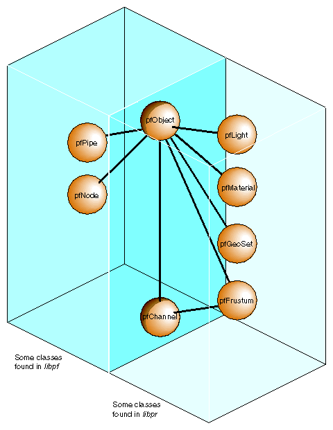
IRIS Performer objects are divided into two groups: those found in the libpf library and those found in the libpr library. These two groups of objects have some common attributes, but also differ in some respects.
While IRIS Performer only uses single inheritance, some objects encapsulate others, hiding the encapsulated object but also providing a functional interface that mimics its original one. For example a pfChannel has a pfFrustum, a pfFrameStats has a pfStats, and a pfPipeWindow has a pfWindow. In these cases, the first object in each pair provides functions corresponding to those of the second. For example, pfFrustum has a routine,
pfMakeSimpleFrust(frust, 45.0f); |
and pfChannel has a corresponding routine,
pfMakeSimpleChan(channel, 45.0f); |
All of the major classes in IRIS Performer are derived from the pfObject class. It unifies the data types by providing common attributes and functions. However, some distinctions remain between libpr objects and libpf objects, due to memory and performance considerations.
The primary attribute of a pfObject is called “user data”; its primary functions are pfDelete(), pfCopy(), and pfPrint().
Each pfObject contains a special pointer to void which is reserved for application use. This pointer can be set with pfUserData() to point to a user-supplied data structure. This user structure usually further describes the pfObject by adding attributes that make sense to the application.Both libpf and libpr objects have user data pointers.
Most kinds of data objects in IRIS Performer can be placed in a hierarchical scene graph, using instancing (see “Instancing” in Chapter 5) when an object is referenced multiple times. Scene graphs can become quite complex, which can cause problems if you're not careful. Deleting objects can be a particularly dangerous operation, for example, if you delete an object that another object still references.
Reference counting provides a bookkeeping mechanism that makes object deletion safe: an object is never deleted if its reference count is greater than zero. Only libpr objects have an explicit reference count. In libpf, pfNodes are reference-counted by their parents in the scene graph, and all other libpf objects (such as pfChannels and pfPipes) have no reference count because you cannot currently delete them.
All libpr objects (such as pfGeoState and pfMaterial) have a reference count that specifies how many other objects refer to it. A reference is made whenever an object is attached to another using the IRIS Performer routines shown in Table 2-2.
Table 2-2. Routines that Modify libpr Object Reference Counts
Routine | Action |
|---|---|
Attaches a pfGeoState to a pfGeoSet | |
Attaches a state structure (such as a pfMaterial) to a pfGeoState | |
Attaches a pfHighlight to a pfGeoSet | |
Attaches a detail pfTexture to a base pfTexture | |
Attaches attribute and index arrays to a pfGeoSet | |
Attaches an image array to a pfTexture | |
When object A is attached to object B, the reference count of A is incremented. Additionally, if A replaces a previously referenced object C, then the reference count of C is decremented. Example 2-1 demonstrates how reference counts are incremented and decremented.
Example 2-1. Objects and Reference-Counts
pfGeoState *gstateA, *gstateC; pfGeoSet *gsetB; /* Attach gstateC to gsetB. Reference count of gstateC * is incremented. */ pfGSetGState(gsetB, gstateC); /* Attach gstateA to gsetB, replacing gstateC. Reference * count of gstateC is decremented and that of gstateA * is incremented. */ pfGSetGState(gsetB, gstateA); |
This automatic reference counting done by IRIS Performer routines is usually all you'll ever need. However, the routines pfRef(), pfUnref(), and pfGetRef() allow you to increment, decrement, and retrieve the reference count of a libpr object should you wish to do so. (These routines also work with objects allocated by pfMalloc(); see “Memory Allocation” in Chapter 10 for more information).
An object whose reference count is less than or equal to 0 can be deleted with pfDelete(). pfDelete() works for all libpr objects and all pfNodes but not for other libpf objects like pfPipe and pfChannel. pfDelete() first checks the reference count of an object. If the reference count is non-positive, pfDelete() decrements the reference count of all objects that the current object references, then it deletes the current object. pfDelete() doesn't stop here but continues down all reference chains, deleting objects until it finds one whose count is greater than zero. Once all reference chains have been explored, pfDelete returns a boolean indicating whether it successfully deleted the first object or not. Example 2-2 illustrates the use of pfDelete() with libpr.
Example 2-2. Using pfDelete() with libpr Objects
pfGeoState *gstate0, *gstate1; pfMaterial *mtl; pfGeoSet *gset; gstate0 = pfNewGState(arena); /* initial ref count is 0 */ gset = pfNewGSet(arena); /* initial ref count is 0 */ mtl = pfNewMtl(arena); /* initial ref count is 0 */ /* Attach mtl to gstate0. Reference count of mtl is * incremented. */ pfGStateAttr(gstate0, PFSTATE_FRONTMTL, mtl); /* Attach mtl to gstate1. Reference count of mtl is * incremented. */ pfGStateAttr(gstate1, PFSTATE_FRONTMTL, mtl); /* Attach gstate0 to gset. Reference count of gstate0 is * incremented. */ pfGSetGState(gset, gstate0); /* This deletes gset, gstate0, but not mtl since gstate1 is * still referencing it. */ pfDelete(gset); |
Example 2-3 illustrates the use of pfDelete() with libpf.
Example 2-3. Using pfDelete() with libpf Objects
pfGroup *group; pfGeode *geode; pfGeoSet *gset; group = pfNewGroup(); /* initial parent count is 0 */ geode = pfNewGeode(); /* initial parent count is 0 */ gset = pfNewGSet(arena); /* initial ref count is 0 */ /* Attach geode to group. Parent count of geode is * incremented. */ pfAddChild(group, geode); /* Attach gset to geode. Reference count of gset is * incremented. */ pfAddGSet(geode, gset); /* This has no effect since the parent count of geode is 1.*/ pfDelete(geode); /* This deletes group, geode, and gset */ pfDelete(group); |
Some notes about reference counting and pfDelete():
All reference count modifications are locked so that they guarantee mutual exclusion when multiprocessing.
Objects added to a pfDispList don't have their counts incremented due to performance considerations.
In the multiprocessing environment of libpf, the successful deletion of a pfNode doesn't have immediate effect but is delayed one or more frames until all processes in all processing pipelines are through with the node. This accounts for the fact that pfDispLists don't reference-count their objects.
pfUnrefDelete(obj) is shorthand for
pfUnref(obj);
pfDelete(obj);
Objects whose count reaches zero are not automatically deleted by IRIS Performer. You must specifically request that an object be deleted with pfDelete() or pfUnrefDelete().
pfCopy() is currently implemented for libpr (and pfMalloc()) objects only. Object references are copied and reference counts are modified appropriately, as illustrated in Example 2-4.
pfGeoState *gstate0, *gstate1; pfMaterial *mtlA, *mtlB; gstate0 = pfNewGState(arena); gstate1 = pfNewGState(arena); mtlA = pfNewMtl(arena); /* initial ref count is 0 */ mtlB = pfNewMtl(arena); /* initial ref count is 0 */ /* Attach mtlA to gstate0. Reference count of mtlA is * incremented. */ pfGStateAttr(gstate0, PFSTATE_FRONTMTL, mtlA); /* Attach mtlB to gstate1. Reference count of mtlB is * incremented. */ pfGStateAttr(gstate1, PFSTATE_FRONTMTL, mtlB); /* gstate1 = gstate0. The reference counts of mtlA and mtlB * are 2 and 0 respectively. Note that mtlB is NOT deleted * even though its reference count is 0. */ pfCopy(gstate1, gstate0); |
Sometimes you have a pointer to a pfObject but you don't know what it really is—is it a pfGeoSet, a pfChannel, or something else? pfGetType() returns a pfType which specifies the type of a pfObject. This pfType can be used to determine the class ancestry of the object. Another set of routines, one for each class, returns the pfType corresponding to that class, e.g. pfGetGroupClassType() returns the pfType corresponding to pfGroup.
Since pfTypes are most frequently used to answer the question is object A of class B, a helper function pfIsOfType() performs the test without the explicit use of a pfType.
With these functions you can test for class type as shown in Example 2-5.
Example 2-5. General-Purpose Scene Graph Traverser
void
travGraph(pfNode *node)
{
    if (pfIsOfType(node, pfGetDCSClassType()))
        doSomethingTransforming(node);

    /* If 'node' is derived from pfGroup then recursively
     * traverse its children */
    if (pfIsOfType(node, pfGetGroupClassType()))
        for (i = 0; i < pfGetNumChildren(node); i++)
            travGraph(pfGetChild(node, i));
}
|
Because IRIS Performer allows subclassing of built-in types, when decisions are made based on the type of an object, it is usually better to use pfIsOfType() to test the type of an object rather than to test for the strict equality of the pfTypes. Otherwise the code will not have reasonable default behavior with file loaders or applications which use subclassing.
While the pfType returned from pfGetType() is useful to programs, it doesn't mean much to humans. pfGetTypeName() returns a null-terminated ASCII string that clearly identifies an object's type. For a pfDCS, for instance, pfGetTypeName() returns the string “pfDCS”.
[1] In recognition of the ingenuity of this system, IRIS Performer includes a star database with the locations and magnitudes of the 3010 brightest stars as seen from earth. View the file “/usr/share/Performer/data/3010.star” with perfly while contemplating the engineering effort required to accurately embed those 966 ball bearings.