This chapter describes how to manage the display operations of a visual simulation application to maintain the desired frame rate and visual performance level.In addition this chapter covers advanced topics including multiprocessing and shared memory management.
A frame is the period of time in which all processing must be completed before updating the display with a new image, for example, a frame rate of 60Hz means the display is updated 60 times per second and the time extent of a frame is 16.7ms. The ability to fit all processing within a frame depends on several variables, some of which are:
the number of pixels being filled
the number of transformations and modal changes being made
the amount of processing required to create a display list for a single frame
the quantity of information being sent to the graphics subsystem
Through intelligent management of Silicon Graphics CPU and graphics hardware, IRIS Performer minimizes the above variables in order to achieve the desired frame rate. However, in some cases, peak frame rate is less important than a fixed frame rate. Fixed frame rate means that the display is updated at a consistent, unvarying rate. While a simple step towards achieving a fixed frame rate is to reduce the frame rate expectation, we shall explore other (less Draconian) mechanisms in this chapter that do not adversely impact frame rates.
As discussed in the following sections, IRIS Performer lets you select the frame rate and has built-in functionality to maintain that frame rate and control overload situations when the draw time exceeds or grows uncomfortably close to a frame time. While these methods can be effective, they do require some cooperation from the run-time database. In particular, databases should be modeled with levels-of-detail and be spatially arranged.
IRIS Performer is designed to run at the fixed frame rate as specified by pfFrameRate(). Selecting a fixed frame rate does not in itself guarantee that each frame can be completed within the desired time. It is possible that some frames might require more computation time than is allotted by the frame rate. By taking too long, these frames cause dropped or skipped frames. A situation in which frames are dropped is called an overload or overrun situation. A system that is close to dropping frames is said to be in stress.
The first step towards achieving a frame rate is to make sure that the scene can be processed in less than a frame's time—hopefully much less than a frame's time. Although minimizing the processing time of a frame is a huge effort, rife with tricks and black magic, certain techniques stand out as IRIS Performer's main weapons against slothful performance:
Multiprocessing. The use of multiple processes on multi-CPU systems can drastically increase throughput.
View culling. By trivially rejecting portions of the database outside the viewing volume, performance can be increased by orders of magnitude.
State sorting. Many graphics pipelines are sensitive to graphics mode changes. Sorting a scene by graphics state greatly reduces mode changes, increasing the efficiency of the hardware.
Level-of-detail. Objects that are far away project to a relatively small area of the display so fewer polygons can be used to render the object without substantial loss of image quality. The overall result is fewer polygons to draw and improved performance.
Multiprocessing and level-of-detail is discussed in this chapter while view culling and state sorting are discussed in Chapter 6, “Database Traversal.” More information on sorting in the context of performance tuning can be found in Chapter 13, “Performance Tuning and Debugging.”
Frame intervals are fixed periods of time but frame processing is variable in nature. Because things change in a scene, such as when objects come into the field of view, frame processing cannot be fixed. In order to maintain a fixed frame rate, the average frame processing time must be less than the frame time so that fluctuations don't exceed the selected frame time. Alternately, the scene complexity can be automatically reduced or increased so that the frame rate stays within a user-defined “sweet spot”. This mechanism requires that the scene be modeled with levels-of-detail (pfLOD nodes).
Each frame, IRIS Performer calculates the system load for each frame. Load is calculated as the percentage of the frame period it took to process the frame. Then if the default IRIS Performer fixed frame rate mechanisms are enabled, load is used to calculate system stress, which is in turn used to adjust the level of detail (LOD) of visible models. LOD management is IRIS Performer's primary method of managing system load.
Table 7-1 shows the IRIS Performer functions for controlling frame processing.
Table 7-1. Frame Control Functions
Function | Description |
|---|---|
Set the desired frame rate. | |
Synchronize processing to frame boundaries. | |
Initiate frame processing. | |
Control frame boundaries. | |
Control how stress is applied to LOD ranges. | |
Manually control the stress value. | |
Determine the current system load. | |
Control how LOD is performed, including global LOD adjustment and blending (fade). |
Figure 7-1 shows a frame-timing diagram that illustrates what occurs when frame computations are not completed within the required interval. The solid vertical lines in Figure 7-1 represent frame-display intervals. The dashed vertical lines represent video refresh intervals.
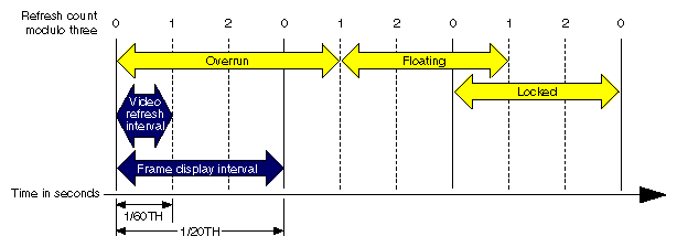
In this example, the video scan rate is 60 Hz and the frame rate is 20 Hz. With the video hardware running at 60 Hz, each of the 20 Hz frames should be scanned to the video display three times, and the system should wait for every third vertical retrace signal before displaying the next image. The numbers across the top of the figure represent the refresh count modulo three. New images are displayed on refreshes whose count modulo three is zero, as shown by the solid lines.
In the first frame of this example, the new image isn't yet completed when the third vertical retrace signal occurs; the same image must therefore be displayed again during the next interval. This situation is known as frame overrun, because the frame computation time extends past a refresh boundary.
Because of the overrun, the frame and refresh interval timing is no longer synchronized; it's out of phase. A decision must be made either to display the same image for the remaining two intervals, or to switch to the next image even though the refresh isn't aligned on a frame boundary. The frame-rate control mode, discussed in the next section, determines which choice is selected.
Knowing that the situation illustrated in Figure 7-1 is a possibility, you can specify a frame control mode to indicate what you would like the system to do when a frame overrun occurs.
To specify a method of frame-rate control, call pfPhase(). There are three available choices:
Free run without phase control (PFPHASE_FREE_RUN) tells the application to run as fast as possible—to display each new frame as soon as it's ready, without attempting to maintain a constant frame rate.
Free run without phase control but with a limit on the maximum frame rate (PFPHASE_LIMIT) tells the application to run no faster than a specified rate.
Fixed frame rate with floating phase (PFPHASE_FLOAT) allows the drawing process to display a new frame (using swapbuffers(3G)) at any time, regardless of frame boundaries.
Fixed frame rate with locked phase (PFPHASE_LOCK) requires the draw process to wait for a frame boundary before displaying a new frame.
The simplest form of frame-rate control, called free-running, is to have no control at all. This uncontrolled mode draws frames as quickly as the hardware is able to process them. In free-running mode, the frame rate may be 60 Hz in the areas of low database complexity, but could drop to a slower rate in views that place greater demand on the system. Use pfPhase(PFPHASE_FREE_RUN) to specify a free-running frame rate.
In applications in which real-time graphics provide the majority of visual cues to an observer, the variable frame rates produced by the free-running mode may be undesirable. The variable lag in image update associated with variable frame rate can lead to motion sickness for the simulation participants, especially in motion platform-based trainers or immersive head-mounted displays. For these and other reasons it is usually preferable to maintain a steady, consistent frame-update rate.
Assume that the overrun frame in Figure 7-1 completes processing during the next refresh period, as shown. After the overrun frame, the simulation is still running at the chosen 20-Hz rate and is updating at every third vertical retrace. If a new image is displayed at the next refresh, its start time lags by 1/60th of a second, and therefore it is out of phase by that much.
Subsequent images are displayed when the refresh count modulo three is one. As the simulation continues and additional extended frames occur, the phase continues to drift. This mode of operation is called floating phase, as shown by the frame in Figure 7-1 labeled Floating. Use pfPhase(PFPHASE_FLOAT) to select floating-phase frame control.
The alternative to displaying a new image out of phase is to display the old image for the remainder of the current update period, then change to the new image at the normal time. This locked phase extends each frame overrun to an integral multiple of the selected frame time, making the overrun more evident but also maintaining phase throughout the simulation. This timing is shown by the frame in Figure 7-1 labeled Locked. Although this mode is the most restrictive, it is also the most desirable in many cases. Use pfPhase(PFPHASE_LOCK) to select phase-locked frame control.
For example, a 20-Hz phase-locked frame rate is selected by specifying:
pfPhase(PFPHASE_LOCK); pfFrameRate(20.0f); |
These specifications prevent the system from switching to a newly computed image until a display period of 1/20th second has passed from the time the previous image was displayed. The frame rate remains fixed even when the Geometry Pipeline finishes its work in less time. Fixed frame-rate display therefore involves setting the desired frame rate and selecting one of the two fixed-frame-rate control modes.
When multiple frame times elapse during the rendering of a single frame, the system must choose which frame to draw next. If the per-frame display lists are processed in strict succession even after a frame overrun, the visual image slowly recedes in time and the positional correlation between display and simulation is lost. To avoid this problem, only the most recent frame definition received by the draw process is sent to the Geometry Pipeline, and all intervening frame definitions are abandoned. This is known as dropping or skipping frames and is performed in both of the fixed frame-rate modes.
Because the effects of variable frame rates, phase variance, and frame dropping are distracting, you should choose a frame rate with care. Steady frame rates are achieved when the frame time allows the worst-case view to be computed without overload. The structure of the visual database, particularly in terms of uniform “complexity density,” can be important in maximizing the system frame rate. See “Organizing a Database for Efficient Culling” in Chapter 6 and Figure 6-3 for examples of the importance of database structure.
Maintaining a fixed frame rate involves managing future system load by adjusting graphics display actions to compensate for varying past and present loads. The theory behind load management and suggested methods for dealing with variable load situations are discussed in the “Level-of-Detail Management” section of this chapter.
Example 7-1 demonstrates a common approach to frame control. The code is based on part of the main.c source file used in the perfly sample application.
Example 7-1. Frame Control Excerpt
/* Set the desired frame rate. */
pfFrameRate(ViewState->frameRate);

/* Set the MP synchronization phase. */
pfPhase(ViewState->phase);

/* Application main loop */
while (!SimDone())
{
    /* Sleep until next frame */
    pfSync();

    /* Should do all latency-critical processing between
     * pfSync() and pfFrame().  Such processing usually
     * involves changing the viewing position.
     */
    PreFrame();

    /* Trigger cull and draw processing for this frame. */
    pfFrame();

    /* Perform non-latency-critical simulation updates. */
    PostFrame();
}
|
All graphics systems have finite capabilities that affect the number of geometric primitives that can be displayed per frame at a specified frame rate. Because of these limitations, maximizing visual cues while minimizing the polygon count in a database is often an important aspect of database development. Level-of-detail processing is one of the most beneficial tools available for managing database complexity for the purpose of improving display performance.
The basic premise of LOD processing is that objects that are barely visible, either because they are located a great distance from the eyepoint or because atmospheric conditions reduce visibility, don't need to be rendered in great detail in order to be recognizable. This is in stark contrast to brutishly mandating that all polygons be rendered regardless of their contribution to the visual scene. Both atmospheric effects and the visual effect of perspective decrease the importance of details as range from the eyepoint increases. The predominant visual effect of distance is the perspective foreshortening of objects, which makes them appear to shrink in size as they recede into the distance.
To save rendering time, objects that are visually less important in a frame can be rendered with less detail. The LOD approach to optimizing the display of complex objects is to construct a number of progressively simpler versions of an object and to select one of them for display as a function of range.
This requires you to create multiple models of an object with varying levels of detail. You also must supply a rule to determine how much detail is appropriate for a given distance to the eyepoint. The sections that follow describe how to create multiple LOD models and how to control when the changeover to a different LOD occurs.
Most objects comprise smaller objects that become visually insignificant at ranges where the conglomerate object itself is still quite prominent. For example, a complex model of an automobile might have door handles, side- and rear-view mirrors, license plates, and other small details.
A short distance away, these features may no longer be visible, even though the car itself is still a visually significant element of the scene. It is important to realize that as a group, these small features may contain as many polygons as the larger car itself, and thus have a detrimental effect on rendering speed.
You can construct two LOD models simply by providing one model that contains all of the detailed features and another model that contains only the car body itself and none of the detailed features. A more sophisticated scheme uses multiple LOD models that are grouped under an LOD node.
Figure 7-2 shows an LOD node with multiple children numbered 1 through n. In this case, the model named LOD 1 is the most detailed model and models LOD 2 through LOD n represent progressively coarser models. Each of these LOD models might contain children that also have LOD components. Associated with the LOD node is a list of ranges that define the distance at which each model is appropriate to display. There is no limit to the number of levels of detail that can be used.
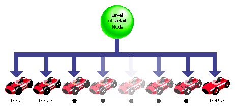
The object can be transformed as needed. During the culling phase of frame processing, the distance from the eyepoint to the object is computed and used (with other factors) to select which LOD model to display.
The IRIS Performer pfLOD node contains a value known as the center of LOD processing. The LOD center point is an x, y, z location that defines the point used in conjunction with the eyepoint for LOD range-switching calculations, as described in the “Level-of-Detail Range Processing” section of this chapter.
Figure 7-3 shows an example in which multiple LOD models grouped under a parent LOD node are used to represent a toy racecar.
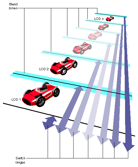
Figure 7-3 demonstrates that each car in a row of identical cars placed at increasing range from the eyepoint is drawn using a different child of the tree's LOD node.
The double-ended arrows indicate a switch range for each level of detail. When the car is closer to the eyepoint than the first range, nothing is drawn. When the car is between the first and second ranges, LOD 1 is drawn. When the car is between the second and third ranges, LOD 2 is drawn.
This range bracketing continues until the final range is passed, at which point nothing is drawn. The pfLOD node's switch range list contains one more entry than the number of child nodes to allow for this range bracketing.
IRIS Performer provides the ability to specify a blend zone for each switch between LOD models. Such that pfLOD nodes now also hold a list of these transition distances over which Performer should `blend' between neighboring LODs. These blend zones will be discussed in more detail in “Level-of-Detail Transition Blending”.
IRIS Performer 2.0 supports a new concept along with the aforementioned standard LOD node which contains switch ranges and transition zones. This new concept is one of an LOD state—the pfLODState. A pfLODState is an essence a way of creating classes or priorities among LODs. A pfLODstate contains eight parameters used to modify four different ways in which Performer calculates LOD switch ranges and LOD transition distances. LOD states contain the following parameters:
Scale for LODs switch Ranges.
Offset for LODs switch Ranges.
Scale for the effect of Stress of switch Ranges.
Offset for the effect of Stress on switch Ranges.
Scale for the transition distances per LOD switch
Offset for the transition distances per LOD switch
Scale for the effect of Stress on transition distances
Offset for the effect of Stress on transition distances
These LOD states can then be attached to either single or multiple LOD nodes such that the LOD behavior of groups or classes of objects can be different and be easily modified. The reference pages for pfLODLODState() and pfLODLODStateIndex() contain detailed information on how to attach pfLODStates.
LOD states are useful because in a particular scene there often exists an object of focus such as a sign, a target, or some other object of particular visual significance that needs to be treated specially with regard to visual importance and thus LOD behavior. It stands to reason, that this particular object (or small group of objects) should be at the highest detail possible despite being farther away than other elements in the scene which might not be as visually significant. In fact, it might be feasible to diminish the detail of these less important objects (like rocks and trees) in favor of the other more important objects (despite these objects being further relatively in range). In this case one would just create two LOD states. The first would be for the important objects and would effectively disable the effect of stress on these nodes as well as scale the switch ranges such that the object(s) would maintain more detail for further ranges. The second LOD state would be used to make the objects of less importance be more responsive to system stress and possibly scale their switch ranges such that they would show even less detail than normal. In this way, LOD states allow biasing among different LODs to maintain desirable rendering speeds while maintaining the visual integrity of various objects depending on their subjective importance (rather than solely on their current visual significance).
In some multichannel applications, LOD states are used to control the action of LODs in different viewing channels that have different visual significance criteria—for instance one channel might be a normal channel while a second might represent an infra-red display. Rather than simple use of LOD states, it is also possible to specify a list of LOD states to a channel and use indexes from this list for particular LODs (via pfChanLODStateList() and pfLODLODStateIndex()). In this way, in the normal channel a car's geometry might be particularly important while in the infra-red channel, the hot exhaust of the same car might be much more important to observe. This type of channel dependent LOD can be set up by using two distinct and different LOD states for the same index in the lists of LOD states specified for unique channels.
Note that because IRIS Performer performs LOD calculations in a range squared space as much as possible for efficiency reasons, LOD computation becomes more costly when LOD states contain scales that are not equal to 1.0 or offsets not equal to 0.0 for transitions or switch ranges—these offsets force IRIS Performer to perform otherwise avoidable square roots calculations in order to correctly calculate the effects of scale and offset on the LOD.
The LOD switch ranges present in LOD nodes are processed before being used to make the level of detail selection. The goal of range setting is to switch LODs as objects reach certain levels of perceptibility. The size of a channel in pixels, the field of view used in viewing, and the distance from the observer to the display surface all affect object perceptibility.
IRIS Performer uses a channel size of 1024x1024 pixels and a 45-degree field of view as the basis for calculating LOD switching ranges. The screen space size of a channel and the current field of view are used to compute an LOD scale factor that is updated whenever the channel size or the field of view changes.
There is an additional global LOD scale factor that can be used to adjust switch ranges based on the relationship between the observer and the display surface. The default global scale factor is 1.
Note that LOD switch ranges are also effected by LOD states that have been attached to either a particular LOD or to a channel that contains the LOD. These LOD states provide the mechanism to apply both a scale and an offset for an LODs switch ranges and to the effect of system stress on those switch ranges. See “Level of Detail States” for more information of pfLODStates.
Ultimately a LODs switch range without regard to system stress can be computed as follows:
    switch_range[i] =
        (range[i] *
            LODStateRangeScale *
            ChannelLODStateRangeScale +
            LODStateRangeOffset +
            ChannelLODStateRangeOffset) *
        ChannelLODScale *
        ChannelSizeAndFOVFactor;
|
If IRIS Performer channel stress processing is active, the computed range is modified as follows:
    switch_range[i] *=
        (ChannelLODStress *
        LODStateRangeStressScale *
        ChannelLODStateRangeStressScale +
        LODStateRangeStressOffset +
        ChannelLODStateRangeStressOffset);
|
Example 7-2 illustrates how to set LOD ranges. The code in this example is derived from /usr/share/Performer/src/sample/apps/C/lod/lod.c, the main source module for the sample program lod.
Example 7-2. Setting LOD Ranges
/* setLODRanges() -- sets the ranges for the LOD node. The
 * ranges from 0 to NumLODs are equally spaced between min
 * and max.  The last range, which determines how far you
 * can get from the object and still see it, is set to
 * visMax.
 */
void
setLODRanges(pfLOD *lod,float min, float max, float visMax)
{
    int i;
    float range, rangeInc;

    rangeInc = (max - min)/(ViewState->shellLOD + 1);
    for (range = min, i = 0; i < ViewState->shellLOD; i++)
    {
        ViewState->range[i] = range;
        pfLODRange(lod, i, range);
        range += rangeInc;
    }
    ViewState->range[i] = visMax;
    pfLODRange(lod, i, visMax);
}

/* generateShellLODs() -- creates shell LOD nodes according
 * to the parameters specified in the shared data structure.
 */
void
generateShellLODs(void)
{
    int i;
    pfGroup *grp;
    pfVec4 clr;
    long numLOD = ViewState->shellLOD;
    long numPnts = ViewState->shellPnts;
    long numPcs = ViewState->shellPcs;

    for (i = 1; i <= numLOD; i++)
    {
        if (ViewState->shellColor == SHELL_COLOR_SING)
            pfSetVec4(clr, 0.9f, 0.1f, 0.1f, 1.0f);
        else
            /* set the color.  highest level = RED;
             * middle LOD = GREEN; lowest LOD = BLUE
             */
            pfSetVec4(clr,
                  (i <= (long)floor((double)(numLOD/2.0f)))?
                     (-2.0f/numLOD) * i + 1.0f + 2.0f/numLOD:
                     0.0f,
                  (i <= (long)floor((double)(numLOD/2)))?
                     (2.0f/numLOD) * (i - 1):
                     (-2.0f/numLOD) * i + 2.0f,
                  (i <= (long)floor((double)(numLOD/2)))?
                     0.0f:
                     (2.0f/numLOD) * i - 1.0f,
                  1.0f);

        /* build a shell GeoSet */
        grp = createShell(numPcs, numPnts,
                          ViewState->shellSweep, &clr,
                          ViewState->shellDraw);
        normalizeNode((pfNode *)grp);

        /* add geode as another level of detail node */
        pfAddChild(ViewState->LOD, grp);

        /* simplify the geometry, but don't have less than
         * 4 points per circle or less than 3 pieces */
        numPnts = (numPnts > 7) ? numPnts-4 : 4;
        numPcs = (numPcs > 6) ? numPcs-4 : 3;
    }
}

...
    ViewState->LOD = pfNewLOD();

    generateShellLODs();

    /* get the LOD's extents */
    pfGetNodeBSphere(ViewState->LOD, &(ViewState->bSphere));
    pfLODCenter(ViewState->LOD, ViewState->bSphere.center);
    /* set ranges for LODs; there should be (num LODs + 1)
     * range entries */
    setLODRanges(ViewState->LOD, ViewState->minRange,
                 ViewState->maxRange, ViewState->max);
|
An undesirable effect called popping occurs when the sudden transition from one LOD to the next LOD is visually noticeable. This distracting image artifact can be ameliorated with a slight modification to the normal LOD-switching process.
In this modified method a transition per LOD switch is established rather than making a sudden substitution of models at the indicated switch range. These transitions specify distances over which to blend between the previous and next LOD. These zones are considered to be centered at the specified LOD switch distance, as shown by the horizontal shaded bars of Figure 7-3. Note that Performer limits the transition distances to be equal to the shortest distance between the switch range and the two neighboring switch ranges. For more information, see the pfLODTransition() reference page.
As the range from eyepoint to LOD center-point transitions the blend zone, each of the neighboring LOD levels is drawn by using transparency to composite samples taken from the present LOD model with samples taken from the next LOD model. For example, at the near, center, and far points of the transition blend zone between LOD 1 and LOD 2, samples from both LOD 1 and LOD 2 are composited until the end of the transition zone is reached, where all the samples are obtained from LOD 2.
Table 7-2 lists the transparency factors used for transitioning from one LOD range to another LOD range.
Table 7-2. LOD Transition Zones
Distance | LOD 1 | LOD 2 |
|---|---|---|
Near edge of blend zone | 100% opaque | 0% opaque |
Center of blend zone | 50% opaque | 50% opaque |
Far edge of blend zone | 0% opaque | 100% opaque |
LOD transitions are made smoother and much less noticeable by applying a blending technique rather than making a sudden transition. Blending allows LOD transitions to look good at ranges closer to the eye than LOD popping allows. Decreasing switch ranges in this way improves the ability of LOD processing to maximize the visual impact of each polygon in the scene without creating distracting visual artifacts.
The benefits of smooth LOD transition have an associated cost. The expense lies in the fact that when an object is within a blend zone, two versions of that object are drawn. This causes blended LOD transitions to increase the scene polygon complexity during the time of transition. For this reason, the blend zone is best kept to the shortest distance that avoids distracting LOD-popping artifacts. Currently, fade level of detail is supported only on RealityEngine™ graphics systems.
Note that the actual `blend' or `fade' distance used by Performer can also be adjusted by the LOD priority structures called pfLODStates. pfLODStates hold an offset and scale for the size of transition zones as well as an offset and scale for how system stress can affect the size of the transition zones. See “Level of Detail States” for more information on pfLODStates.
Note also, that there exists a global LOD transition scale on a per channel basis that can affect all transition distances uniformly.
Thus for an LOD with 5 switch ranges R0, R1, R2, R3, R4 to switch between four models (M0, M1, M2, M3), there are 5 transition zones T0 (fade in M0), T1 (blend between M0 and M1), T2 (blend between M1 and M2), T3 (blend between M2 and M3), T4 (fade out M3). The actual fade distances (without regard to channel stress) are as follows.
    fadeDistance[i] =
        (transition[i] *
            LODStateTransitionScale *
            ChannelLODStateTransitionScale +
            LODStateTransitionOffset +
            ChannelLODStateTransitionOffset) *
        ChannelLODFadeScale;
|
If Performer management of channel stress is turned on then the above fade distance is modified as follows:
    fadeDistance[i] /=
        (ChannelStress *
        LODStateTransitionStressScale *
        ChannelLODStateTransitionStressScale +
        LODStateTransitionStressOffset +
        ChannelLODStateTransitionStressOffset);
|
In creating LOD models and transitions for objects, it's often safe to assume that the entire model should transition at the same time. It's quite reasonable to make features of an automobile such as door handles disappear from the scene at the same time even when the passenger door is slightly closer than the driver's door. It is much less clear that this approach would work for very large objects such as an aircraft carrier or a space station, and it's clearly not acceptable for objects that span a large extent, such as a terrain surface.
Attempts to handle large-extent objects with discrete LOD tools focus on breaking the big object into myriad small objects and treating each small object independently. This works in some cases but often fails at the junction between two or more independent objects where cracks or seams exist when different detail levels apply to the objects. Some terrain processing systems have attempted to provide a hierarchy of crack filling geometry that is enabled based on the LOD selections of two neighboring terrain patches. This “digital grout” becomes untenable when more than a few patches share a common vertex.
An alternate approach—the active surface definition—treats the entire terrain as a single connected (and coherent) surface. The essence of the approach is that a triangle representing terrain either is judged to be sufficiently accurate or is recursively subdivided. The general manner of subdivision is to introduce one or more vertices along the sides of the original triangle. Connecting these new vertices to make triangles leads to the subdivision of the original triangle into multiple triangles. After subdivision, the algorithm perturbs the vertex positions. If the resulting triangles are not yet sufficiently fine, the subdivision process is applied to each one in turn based on range and other fidelity criteria.
Terrain level of detail using an interpolative active surface definition is a restricted form of the more general notion of object morphing. Morphing of models such as the car in a previous example can simply involve scaling a small detail to a single point and then removing it from the scene. Morphing is possible even when the topologies of neighboring pairs do not match. Both models and terrain can have vertex, normal, color, and appearance information interpolated between two or more representations. The advantages of this approach include: reduced graphics complexity since blending is not used, constant intersection truth for collision and similar tasks, and monotonic database complexity that makes system load management much simpler.
Because the effects of variable image update rates can be objectionable, many simulation applications are designed to operate at a fixed frame rate. One approach to selecting this fixed frame rate is to select an update rate constrained by the most complex portion of the visual database. Although this conservative approach may be acceptable in some cases, IRIS Performer supports a more sophisticated approach using dynamic LOD scaling.
Using multiple LOD models throughout a database provides the traversal system with a parameter that can be used to control the polygonal complexity of models in the scene. The complexity of database objects can be reduced or increased by adjusting a global LOD range multiplier that determines which LOD level is drawn.
Using this facility, a closed-loop control system can be constructed that adjusts the LOD-switching criteria based on the system load, also called stress, in order to maintain a selected frame rate.
Figure 7-4 illustrates a stress-processing control system.

In Figure 7-4, the desired and actual frame times are compared by the stress filter. Based on the user-supplied stress parameters, the stress filter adjusts the global LOD scale factor by increasing it when the system is overloaded and decreasing it when the system is underloaded. In this way, the system load is monitored and adjusted before each frame is generated.
The degree of stability for the closed-loop control system is an important issue. The ideal situation is to have a critically damped control system—that is, one in which just the right amount of control is supplied to maintain the frame rate without introducing undesirable effects. The effects of overdamped and underdamped systems are visually distracting. An underdamped system oscillates, causing the system to continuously alternate between two different LOD models without reaching equilibrium. Overdamped systems may fail to react within the time required to maintain the desired frame rate. In practice, though, dynamic load management works well, and simple stress functions can handle the slowly changing loads presented by many databases.
The default stress function is controlled with user-selectable parameters. These parameters are set using the function pfChanStressFilter().
The default stress function is implemented by the code fragment in Example 7-3.
Example 7-3. Default Stress Function
/* current load */
curLoad = drawTime * frameRate * frameFrac;

/* integrated over time */
if (curLoad < lowLoad)
    stressLevel -= stressParam * stressLevel;
else
if (curLoad > highLoad)
    stressLevel += stressParam * stressLevel;

/* limited to desired range */
if (stressLevel < 1.0)
    stressLevel = 1.0;
else
if (stressLevel > maxStress)
    stressLevel = maxStress;
|
The parameters lowLoad and highLoad define a “comfort zone” for the control system. The first if-test in the code fragment demonstrates that this comfort zone acts as a dead band. Instantaneous system load within the bounds of the dead band doesn't result in a change in the system stress level. If the size of the comfort zone is too small, oscillatory distress is the probable result. It is often necessary to keep the highLoad level below the 100% point so that blended LOD transitions don't drive the system into overload situations.
For those applications in which the default stress function is either inappropriate or insufficient, you can compute the system stress yourself and then set the stress load factor. Your filter function can access the same system measures that the default stress function uses, but it's also free to keep historical data and perform any feedback-transfer processing that application-specific dynamic load management may require.
The primary limitation of the default stress function is that it has a reactive rather than predictive nature. One of the major advantages of user-written stress filters is their ability to predict future stress levels before increased or decreased load situations reach the pipeline. Often the simulation application knows, for example, when a large number of moving models will soon enter the viewing frustum. If their presence is anticipated, then stress can be artificially increased so that no sudden LOD changes are required as they actually enter the field of view.
This section describes an advanced topic that applies only to systems with more than one CPU. If you don't have a multiple-CPU system, you may want to skip this section.
IRIS Performer uses multiprocessing to increase throughput for both rendering and intersection detection. Multiprocessing can also be used for tasks that run asynchronously from the main application like database management. Although IRIS Performer hides much of the complexity involved, you need to know something about how multiprocessing works in order to use multiple processors well.
Recall from Chapter 3 that an IRIS Performer application renders images using one or more pfPipes as independent software-rendering pipelines. The flow through the rendering pipeline can be modeled using these functional stages:
| Intersection | Test for intersections between segments and geometry to simulate collision detection or line-of-sight for example. | |
| Application | Do requisite processing for the visual simulation application, including reading input from control devices, simulating the vehicle dynamics of moving models, updating the visual database, and interacting with other networked simulation stations. | |
| Cull | Traverse the visual database and determine which portions of it are potentially visible, perform level-of-detail selection for models with multiple representations, and build sorted, optimized display list for the draw stage. | |
| Draw | Issue graphics library commands to a Geometry Pipeline in order to create an image for subsequent display. |
You can partition these stages into separate parallel processes in order to distribute the work among multiple CPUs. Depending on your system type and configuration, you can use any of several available multiprocessing models.
Use pfMultiprocess() to specify which functional stages, if any, should be forked into separate processes. The multiprocessing mode is actually a bitmask where each bit indicates that a particular stage should be configured as a separate process. For example, the bit PFMP_FORK_DRAW means the draw stage should be split into its own process. Table 7-3 lists some convenience tokens that represent common multiprocessing modes:
Table 7-3. Multiprocessing Models
Model Name | Description |
|---|---|
Combine the application, cull, and draw stages into a single process. In this model, all of the stages execute within a single frame period. This is the minimum-latency mode of operation. | |
|
or | Combine the cull and draw stages in a process that is separate from the application process. This model provides a full frame period for the application process, while culling and drawing share this same interval. This mode is appropriate when the host's simulation tasks are extensive but graphic demands are light, as might be the case when complex vehicle dynamics are performed but only a simple dashboard gauge is drawn to indicate the results. |
|
or | Combine the application and cull stages in a process that is separate from the draw process. This mode is appropriate for many simulation applications when application and culling demands are light. It allocates a full CPU for drawing and has the APP and CULL stages share a frame period. Like the PFMP_APP_CULLDRAW mode, this mode has a single frame period of pre-draw latency. |
|
or | Perform the application, cull, and draw stages as separate processes. This is the full maximum-throughput multiprocessing mode of IRIS Performer operation. In this mode, each pipeline stage is allotted a full frame period for its processing. Two frame periods of latency exist when using this high degree of parallelism. |
You can also use pfMultiprocess() to specify the method of communication between the cull and draw stages, using the bitmasks PFMP_CULLoDRAW and PFMP_CULL_DL_DRAW.
Setting PFMP_CULLoDRAW specifies that the cull and draw processes for a given frame should overlap—that is, that they should run concurrently. For this to work, the cull and draw stages must be separate processes (PFMP_FORK_DRAW must be true). In this mode the two stages communicate in the classic producer-consumer model, by way of a pfDispList that is configured as a ring (FIFO) buffer; the cull process puts commands on the ring while the draw process simultaneously consumes these commands.
The main benefit of using PFMP_CULLoDRAW is reduced latency, since the number of pipeline stages is reduced by one and the resulting latency is reduced by an entire frame time. The main drawback is that the draw process must wait for the cull process to begin filling the ring buffer.
When the cull and draw stages are in separate processes, they communicate through a pfDispList; the cull process generates the display list, and the draw process traverses and renders it. (The display list is configured as a ring buffer when using PFMP_CULLoDRAW mode, as described in the “Cull-Overlap-Draw Mode” section).
However, when the cull and draw stages are in the same process (as occurs with the PFMP_APPCULLDRAW or PFMP_APP_CULLDRAW multiprocessing models) a display list isn't required and by default one will not be used. Leaving out the pfDispList eliminates overhead. When no display list is used, the cull trigger function pfCull() has no effect; the cull traversal takes place when the draw trigger function pfDraw() is invoked.
In some cases you may want an intermediate pfDispList between the cull and draw stages even though those stages are in the same process. The most common situation that calls for such a setup is multipass rendering, when you want to cull only once but render multiple times. With PFMP_CULL_DL_DRAW enabled, pfCull() generates a pfDispList that can be rendered multiple times by multiple calls to pfDraw().
The intersection pipeline is a two-stage pipeline consisting of the application and the intersection stages. The intersection stage may be configured as a separate process by setting the PFMP_FORK_ISECT bit in the bitmask given to pfMultiprocess(). When configured as such, the intersection process is triggered for the current frame when the application process calls pfFrame(). Then in the special intersection callback set with pfIsectFunc(), you can invoke any number of intersection requests with pfNodeIsectSegs().
The intersection process is asynchronous so that if it does not finish within a frame time it does not slow down the rendering pipeline(s).
By default, IRIS Performer uses a single pfPipe, which in turn draws one or more pfChannels into one or more pfPipeWindows. If you want to use multiple rendering pipelines, as on two- or three-Geometry Pipeline Onyx RealityEngine2 systems, use pfMultipipe() to specify the number of pfPipes required. When using multiple pipelines, the PFMP_APPCULLDRAW and PFMP_APPCULL_DRAW modes are not supported and IRIS Performer defaults to the PFMP_APP_CULL_DRAW multiprocessing configuration. Regardless of the number of pfPipes, there is always a single application process which triggers the rendering of all pipes with pfFrame().
For additional multiprocessing and attendant increased throughput, the CULL stage of the rendering pipeline may be multithreaded. Multithreading means that a single pipeline stage is split into multiple processes, or threads which concurrently work on the same frame. Use pfMultithread() to allocate a number of threads for the cull stage of a particular rendering pipeline.
Cull multithreading takes place on a per-pfChannel basis, that is, each thread does all the culling work for a given pfChannel. Thus, an application with only a single channel will not benefit from multithreading the cull and an application with multiple, equally complex channels will benefit most by allocating a number of cull threads equal to the number of channels. However, it is legal to allocate fewer cull threads if you do not have enough CPUs—in this case the threads are assigned to channels on a need basis.
The multiprocessing model set by pfMultiprocess() is used for each of the rendering pipelines. In programs that configures the application stage as a separate process, all IRIS Performer calls must be made from the process that calls pfConfig() or the results are undefined. Both pfMultiprocess(), pfMultithread(), and pfMultipipe() must be called after pfInit() but before pfConfig(). pfConfig() configures IRIS Performer according to the required number of pipelines and the desired multiprocessing and multithreading modes, forks the appropriate number of processes, and then returns control to the application. pfConfig() should be called only once during each IRIS Performer application.
Figure 7-5 shows timing diagrams for each of the process models. The vertical lines are frame boundaries. Five frames of the simulation are shown to allow the system to reach steady-state operation.
Boxes represent the functional stages and are labeled as follows:
| An | application process for the nth frame | |
| Cn | cull process for the nth frame | |
| Dn | draw process for the nth frame |
Only one of these models can be selected at a time, but they are shown together so that you can compare their structures.
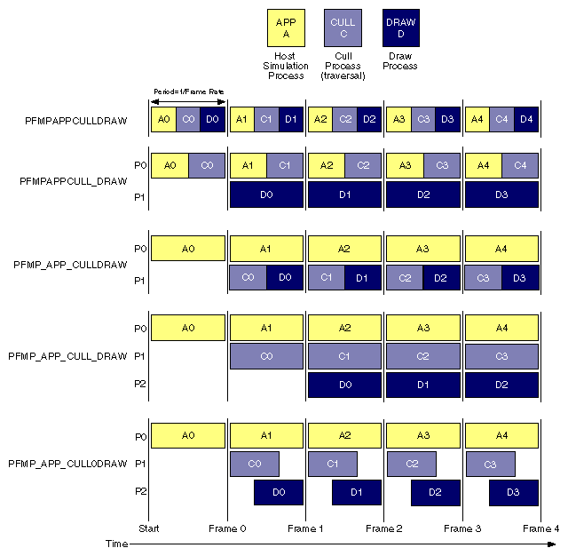
Notice that when a stage is split into its own process, the amount of time available for all stages increases. For example, in the case where the application, cull, and draw stages are 3 separate processes, it is possible for total system performance to be tripled over the single process configuration.
Many databases are too large to fit into main memory. A common solution to this problem is called database paging where the database is divided into manageable chunks on disk and loaded into main memory when needed. Usually chunks are paged in just before they come into view and are deleted from the scene when they are comfortably out of viewing range.
All this paging from disk and deleting from main memory takes a lot of time and is certainly not amenable to maintaining a fixed frame rate. The solution supported by IRIS Performer is asynchronous database paging in which a process, completely separate from the main processing pipeline(s), handles all disk I/O and memory allocations and deletions. To facilitate asynchronous database paging, IRIS Performer provides the pfBuffer structure and the DBASE process.
The database (or DBASE) process is forked by pfConfig() if the PFMP_FORK_DBASE bit was set in the mode given to pfMultiprocess(). The database process is triggered when the application process calls pfFrame() and invokes the user-defined callback set with pfDBaseFunc(). The database process is totally asynchronous. If it exceeds a frame time it does not slow down any rendering or intersection pipelines.
The DBASE process is intended for asynchronous database management when used with pfBuffer.
A pfBuffer is a logical buffer which isolates database changes to a single process, avoiding disastrous collisions on data from multiple processes. In typical use, a pfBuffer is created with pfNewBuffer(), made current with pfSelectBuffer() and merged with the main IRIS Performer buffer with pfMergeBuffer(). While the DBASE process is intended for pfBuffer use, other processes forked by the application may also use different pfBuffers in parallel for multithreaded database management. By ensuring that only a single process uses a given pfBuffer at a given time and following a few scoping rules discussed below, the application can safely and efficiently implement asynchronous database paging
A pfNode is said to have buffer scope or be “in” a particular pfBuffer. This is an important concept because it affects what you can do with a given node. A newly-created node is automatically “in” the currently active pfBuffer until that pfBuffer is merged using pfMergeBuffer(). At that instant, the pfNode is moved into the main IRIS Performer buffer, otherwise known as the application buffer.
A rule in pfBuffer management is that a process may only access nodes that are in its current pfBuffer. As a result, a database process may not directly add a newly created subgraph of nodes to the main scene graph because all nodes in the main scene graph have application buffer scope only—they are isolated from the database pfBuffer. This may seem inconvenient at first but it eliminates catastrophic errors like, for example, the application process traverses a group at the same time you add a child, changing its child list and causing the traversal to chase a bad pointer.
Remedies to the inconveniences stated above are the pfBufferAddChild(), pfBufferRemoveChild() and pfBufferClone() routines. The first two routines are identical to their non-buffer counterparts pfAddChild() and pfRemoveChild() except the buffer versions do not happen immediately. Other functions, pfBufferAdd(), pfBufferInsert(), pfBufferReplace(), and pfBufferRemove(), perform the buffer-oriented delayed-action versions of the corresponding non-buffer pfList functions. In all cases the add, insert, replace, or removal request is placed on a list in the current pfBuffer and is processed later at pfMergeBuffer() time.
pfBufferClone() supports the notion of maintaining a “library” of common objects like trees or houses in a special library pfBuffer. The main database process then clones objects from the library pfBuffer into the database pfBuffer, possibly pfFlatten()ing them for improved rendering performance. pfBufferClone() is identical to pfClone() except the buffer version requires that the source pfBuffer be specified and that all cloned nodes have scope in the source pfBuffer.
We've discussed how to create subgraphs for database paging: create and select a current pfBuffer, create nodes and build the subgraph, call pfBufferAddChild() and finally pfMergeBuffer() to incorporate the subgraph into the application's scene. But what about freeing the memory of old, unwanted subgraphs? For this we turn to pfAsyncDelete().
pfDelete() is the normal mechanism for deleting objects and freeing their associated memory. However, pfDelete() can be a very costly routine since it must traverse, unreference, and register a deletion request for every IRIS Performer object it encounters which has a 0 reference count. pfAsyncDelete(), in conjunction with a forked DBASE process, moves the burden of deletion to the asynchronous database process so that all rendering and intersection pipelines are not adversely affected.
pfAsyncDelete() may be called from any process and places an asynchronous deletion request on a global list that is processed later by the DBASE stage when its trigger routine, pfDBase() is called. A major difference from pfDelete() is that pfAsyncDelete() does not immediately check the reference count of the object to be deleted and so does not return a value indicating whether the deletion was successful or not. At this time there is no way of querying the result of a pfAsyncDelete() request so care should be taken that the object to be deleted has no reference counts or memory leaks will result.
There are some restrictions on which functions can be called from an IRIS Performer process while multiple processes are running. Some specialized processes (such as the process handling the draw stage) can call only a few specific IRIS Performer functions, and can't call any other kinds of functions. This section lists general and specific rules concerning function invocation in the various IRIS Performer and user processes.
In this section, the term “the draw process” refers to whichever process is handling the draw stage, regardless of whether that process is also handling other stages. Similarly, “the cull process” and “the application process” refer to the processes handling the cull and application stages, respectively.
This is a general list of the kinds of routines you can call from each process:
| application | configuration routines, creation and deletion routines, set and get routines, and trigger routines such as pfAppFrame(), pfSync(), pfFrame() | |
| database | creation and deletion routines, set and get routines, pfDBase(), pfMergeBuffer() | |
| cull | pfCull(), pfCullPath(), IRIS Performer graphics routines | |
| draw | pfClearChan(), pfDraw(), pfDrawChanStats(), IRIS Performer graphics routines, graphics library routines |
More specific elaborations:
You should call configuration routines only from the application process, and only after pfInit() and before pfConfig(). pfInit() must be the first IRIS Performer call except for those routines that configure shared memory (see “Memory Allocation” in Chapter 10). Configuration routines don't take effect until pfConfig() is called. These are the configuration routines:
You should call creation routines, such as pfNewChan(), pfNewScene(), and pfAllocIsectData(), only in the application process after calling pfConfig() or in a process which has an active pfBuffer. There is no restriction on creating libpr objects like pfGeoSets and pfTextures.
pfDelete() should only be called from the application or database processes. pfAsyncDelete() may be called from any process.
Read-only routines—that is, the pfGet*() functions—can be called from any IRIS Performer process. However, if a forked draw process queries a pfNode, the data returned will not be frame-accurate. (See “Multiprocessing and Memory”.)
Write routines—functions that set parameters—should be called only from the application process or a process with an active pfBuffer. It is possible to call a write routine from the cull process, but it isn't recommended since any modifications to the database will not be visible to the application process if it is separate from the cull (as when using PFMP_APP_CULLDRAW or PFMP_APP_CULL_DRAW). However, for transient modifications like custom level-of-detail switching, it is reasonable for the cull process to modify the database. The draw process should never modify any pfNode.
IRIS Performer graphics routines should be called only from the cull or draw processes. These routines may modify hardware graphics state. They are the routines which can be captured by an open pfDispList. (See “Display Lists” in Chapter 10.) If invoked in the cull process, these routines are captured by an internal pfDispList and later invoked in the draw process; but if they are invoked in the draw process they immediately affect the current window. These graphics routines can be roughly partitioned into those that
Graphics library routines should be called only from the draw process. Since there is no open display list to capture these commands, an open window is required to accept them.
“Trigger” routines should be called only from the appropriate processes (see Table 7-4).
Table 7-4. Trigger Routines and Associated Processes
Trigger Routine
Process/Context
pfAppFrame
pfSync
pfFrameAPP/main loop
pfPassChanData
pfPassIsectDataAPP/main loop
pfApp
APP/channel APP callback
pfCull
pfCullPathCULL/channel CULL callback
pfDraw
pfDrawBinDRAW/channel DRAW callback
pfNodeIsectSegs
pfChanNodeIsectSegsISECT/callback or APP/main loop
pfDBase
DBASE/callback
User-spawned processes created with sproc() can trigger parallel intersection traversals through multiple calls to pfNodeIsectSegs() and pfChanNodeIsectSegs().
Functions pfApp(), pfCull(), pfDraw(), and pfDBase() are only called from within the corresponding callback specified by pfChanTravFunc() or pfDBaseFunc().
In IRIS Performer, as is often true of multiprocessing systems, memory management is the most difficult aspect of multiprocessing. Most data management problems in an IRIS Performer application can be partitioned into three categories:
Memory visibility. IRIS Performer uses fork(), which—unlike sproc()— generates processes that don't share the same address space. The processes also cannot share global variables that are modified after the fork() call. After calling fork(), processes must communicate through explicit shared memory.
Memory exclusion. If multiple processes read or write the same chunk of data at the same time, consequences can be dire. For example, one process might read the data while in an inconsistent state and end up dumping core while dereferencing a NULL pointer.
Memory synchronization. IRIS Performer is configured as a pipeline where different processes are working on different frames at the same time. This pipelined nature is illustrated in Figure 7-5, which shows that, for instance, in the PFMP_APP_CULL_DRAW configuration the application process is working on frame n while the draw process is working on frame n-2. If, in this case, if we have only a single memory location representing the viewpoint, then it is possible for the application to set the viewpoint to that of frame n and the draw process to incorrectly use that same viewpoint for frame n-2. Properly synchronized data is called frame accurate.
Fortunately, IRIS Performer transparently solves all of the above problems for most IRIS Performer data structures and also provides powerful tools and mechanisms that the application can use to manage its own memory.
As described in “Initializing and Configuring IRIS Performer” in Chapter 3, pfInit() creates a shared memory arena that is shared by all processes spawned by IRIS Performer and all user processes that are spawned from any IRIS Performer process. A handle to this arena is returned by pfGetSharedArena() and should be used as the arena argument to routines that create data that must be visible to all processes. Routines that accept an arena argument are the pfNew*() routines found in the libpr library and the IRIS Performer memory allocator, pfMalloc(). In practice, it is usually safest to create libpr objects like pfGeoSets and pfMaterials in shared memory. libpf objects like pfNodes are always created in shared memory.
Allocating shared memory does not by itself solve the memory visibility problem discussed above. You must also make sure that the pointer that references the memory is visible to all processes. IRIS Performer objects, once incorporated into the database via routines like pfAddGSet(), pfAddChild(), and pfChanScene(), automatically ensure that the object pointers are visible to all IRIS Performer processes.
However, pointers to application data must be explicitly shared. A common way of doing this is to allocate the shared memory after pfInit() but before pfConfig() and to reference the memory with a global pointer. Since the pointer is set before pfConfig() forks any processes, these processes will all share the pointer's value and can thereby access the same shared memory region. However, if this pointer value changes in a process, its value will not change in any other process, since forked processes don't share the same address space.
Even with data visible to all processes, data exclusion is still a problem. The usual solution is to use hardware spin locks so that a process can lock the data segment while reading or writing data. If all processes must acquire the lock before accessing the data, then a process is guaranteed that no other processes will be accessing the data at the same time. All processes must adhere to this locking protocol, however, or exclusion isn't guaranteed.
In addition to a shared memory arena, pfInit() creates a semaphore arena whose handle is returned by pfGetSemaArena(). Locks can be allocated from this semaphore arena by usnewlock() and can be set and unset by ussetlock() and usunsetlock(), respectively.
pfDataPools—named shared memory arenas with named allocation blocks—provide a complete solution to the memory visibility and memory exclusion problems, thereby obviating the need to set global pointers between pfInit() and pfConfig(). For more information about pfDataPools, see “Datapools”.
The techniques discussed thus far don't solve the memory synchronization problem. Performer's libpf library provides a solution in the form of passthrough data. When using pipelined multiprocessing, data must be passed through the processing pipeline so that data modifications reach the appropriate pipeline stage at the appropriate time.
Passthrough data is implemented by allocating a data buffer for each stage in the processing pipeline. Then, at well-defined points in time, the passthrough data is copied from its buffer into the next buffer along the pipeline. This copying guarantees memory exclusion, but you should minimize the amount of passthrough data to reduce the time spent copying.
Allocate a passthrough data buffer for the rendering pipeline using pfAllocChanData(); for data to be passed down the intersection pipeline, call pfAllocIsectData(). Data returned from pfAllocChanData() is passed to the channel cull and draw callbacks that are set by pfChanTravFunc(). Data returned from pfAllocIsectData() is passed to the intersection callback specified by pfIsectFunc().
Passthrough data isn't automatically passed through the processing pipeline. You must first call pfPassChanData() or pfPassIsectData() to indicate that the data should be copied downstream. This requirement allows you to copy only when necessary—if your data hasn't changed in a given frame, simply don't call a pfPass*() routine, and you'll avoid the copy overhead. When you do call a pfPass*() routine, the data isn't immediately copied but is delayed until the next call to pfFrame(). The data is then copied into internal IRIS Performer memory and you're free to modify your passthrough data segment for the next frame.
Modifications to all libpf objects—such as pfNodes and pfChannels—are automatically passed through the processing pipeline, so frame-accurate behavior is guaranteed for these objects. However, in order to save substantial amounts of memory, libpr objects such as pfGeoSets and pfGeoStates don't have frame-accurate behavior; modifications to such objects are immediately visible to all processes. If you want frame-accurate modifications to libpr objects you must use the passthrough data mechanism, use a frame-accurate pfSwitch to select among multiple copies of the objects you want to change or use the pfCycleBuffer memory type described in “CycleBuffers”.