This chapter explains in detail how to use the Module Builder to construct a module. It describes how you:
create a user function for the module
define include files and libraries for the module
create your own Makefiles
define data input and output ports
specify the function arguments and link them to the ports
configure the build environment
use the build options to build and install the completed module
It also includes some examples of user functions for simple modules.
Advanced topics may require programming skills not covered in this guide. As an ordinary user, you can usually skip these passages.
The user function or subroutine is a program that details what you want the module to do. You can write it yourself or use a program that already exists. The user function file contains the algorithm that actually performs the data transformation. It also contains any API subroutines you are using in the module.
You can write the program in C++, C, or Fortran; however, all user functions must export a C-style user interface. Writers of C++ user functions must qualify their routines accordingly. For example, you can qualify a routine called funcName() as
extern “C” funcName() |
 | Note: In the Explorer environment, all files containing C++ code have the suffix .C. |
You can write the user function at any time, but you cannot build the module without it. You can set up other parts of the module, such as the input and output ports and connections, save the module resources, and then pull up the half-finished module and build it later, when the user function is complete. You can also generate a prototype and build the module later.
The Explorer application programming interface (API) is a set of functions in C and corresponding subroutines in Fortran that give the module writer greater control over module behavior. For example, instead of the Module Builder generating code to connect the user function to the ports, the writer can use the API to do so. The writer can also build more complex modules by using the API to make specific calls to other parts of Explorer. The API is described fully in the IRIS Explorer Reference Pages.
| Note: If your user function is written in C++, use the C API. Since C++ is a superset of C, the C API can be called directly by C++. |
If you try to build a geometry module in Fortran, your only access to the Geometry library is through the Explorer API subroutines. If you want to use the Inventor geometry libraries, you must build geometry modules in C or C++.
If you are writing a module, you can use cxScriptCommand to issue scripting commands from within the module. When you call cxScriptCommand, a message transmission and several context switches result, so performance is improved if you can bundle expressions in a single string.
For more information on syntax of cxScriptCommand and the Skm language, refer to Appendix B in the IRIS Explorer User's Guide.
You use the Module Builder to create the module resources file and the control panel for a module and to build and install the module so that it can be launched in the Map Editor.
In general, you should run the Module Builder from the directory in which you want the completed module to reside; otherwise, the module may not build. See “Building and Installing Modules” for more information.
At the shell prompt (%), type:
mbuilder |
The Module Builder main window appears on the screen (see ). If you open the Module Builder without a filename, the main window comes up with default_module_name in the name slot. In this window, you set the variables for the module resources file, a binary file called <modulename>.mres, which contains all the information required to build the module.

The .mres file template is created as you apply the information from each of the Module Builder windows (see “Moving Around the Windows”) and is saved when you first select “Save Resources” from the File menu.
To open the Module Builder and a module at the same time, change to the directory in which the module resides. For example, to look at the structure of an existing Explorer module, such as GenLat, type:
cd /usr/explorer/modules mbuilder GenLat |
The Module Builder opens with the information pertinent to the module displayed in its windows.
Five windows can be opened from the main Module Builder window, but only one besides the main window can be active at a time. If you try to open more than one, a dialogue box appears and tells you which window is already open. The active window may be buried under other windows or it may be iconified. To re-display the open window, click on the corresponding button in the main Module Builder window.
To select a text type-in slot in any of the Module Builder windows, click on the slot. The active slot is outlined in black and has a cursor in it. You can type into the active slot.
When you have entered information in a window, you can use one of the three buttons at the bottom of the window:
| Cancel | Cancels all the information before it can be saved | |
| Apply | Saves the information and leaves the window open | |
| OK | Saves the information and closes the window |
Changes are not incorporated into the module template until you click on Apply or OK.
To save the template as a modulename.mres file, you must use “Save Resources” on the File menu. You should do this often, to avoid losing your work.
Filling out the Module Builder main window is equivalent to setting the variables required by the language compiler and link editor.
the name of an existing module that you want to examine. For example, the command
mbuilder LatToGeom
opens the Module Builder and LatToGeom. As you move through the Module Builder windows, you have access to the module's internal structure, called the module resources.
the name for a new module that does not yet exist, but that you are about to create. The Module Builder main window appears with the new name in the Module Name slot, but all other windows are empty.
If you want to look at a different module resource file or to create another new module, use the File menu in the Module Builder main window. To select another modulename.mres file, click “Open” and select the file from the file browser that appears. To create a new module, select “New.”
Enter the name of a module in the Module name slot (see Figure 2-1). To enter or change the name of a module in the slot, click the text slot to highlight it and type a new name.
Each module name must begin with an alphanumeric character. Since they are UNIX files, you should follow UNIX file-naming conventions.
If you are modifying an existing module to create a new one, you should save the modified resource file with a new module name and leave the original modulename.mres files intact.
| Note: Because you cannot change the source code of an existing Explorer module, the modifications you can make to these modules are very slight; however, you can modify your own modules endlessly, if you wish. |
By default, Explorer saves newly created modules in your working directory. It saves the module in the form of a modulename.mres file when you select:
“Save Resources” from the File menu (saves the contents of the windows as module resources), or
“Build” or “Build & Install” from the Build menu (saves the resources, compiles and links the source code)
Enter the name of the file or files that contain your computational, or user, function in the User Func File text slot. For example, the Gradient3D module has one user function file, called Gradient3D.f.
Your module may use an alternate executable, that is, a user function connected with another module (see “Using the Build Menu” ). If so, don't enter the name of the user function in the User Func File slot; it appears on the Build Options menu.
If the user function is large and complex, you can break it down into smaller sub-functions, each of which is in its own file. In the User Func File slot, list two or more files with a space between each name.
You can mix languages (C++, C, and Fortran), source files (filename.C, filename.c, or filename.f), and object files (filename.o) in this slot. For example, Render, which is a very complex module, uses render.C, event.C, init.C, SoSceneViewer.C, SvManipList.C, cxGeoObject.C, and several other files.
If you use library (.a) files in the User Func File slot, you need to supply your own Makefile in the User Makefile slot (see “User Makefiles”). If you use source or object files, the Module Builder uses standard make rules to determine file dependencies and to build the necessary object files, and you need not supply a Makefile unless you have a specific reason for doing so.
The Makefile generated by the Module Builder has default rules for generating an object file from C, C++, and Fortran source files.
In Explorer, *.inc files have no cpp directives in them at all.To use #include syntax, name your source file *.fi, and the Explorer Makefiles will filter it for you. If your Fortran compiler naturally supports cpp, you can still use *.f. To use include statement syntax, name your source file *.f.
Use of certain data types requires that you explicitly include certain files. If you use cxLattice, you may need to include Typedefs.inc. If you use cxPyramid, you must include cxLattice.inc. If you use DataTypes.inc, however, it includes Typedefs.inc explicitly.
The Module Builder automatically passes the “include” directories such as /usr/explorer/include and /usr/include to the compiler when compiling the module's source code; however, you may want to include directories or files from other places for a particular module.
Use the Includes slot to do this.
Enter the name of each included file as you would list it in a compile command. Use the form -I<directory>; for example, –I../myInclude. The AnimateCamera module (see ) has this include command:
-I$(CXSYSINCLUDE) |
If you include a system-defined variable by itself, it takes the form ${VARIABLE}; for example, ${GEOMETRYINCS}.
You can also use the -D option for variables; for example, the Render module uses -DEXPLORER. For more information on these options, refer to the UNIX cc(1) command.
Some modules, such as those handling graphics, geometry, or mathematical procedures, and those written in Fortran, must be linked to related libraries. Explorer automatically adds certain default libraries into the module Imakefile for Fortran and geometry modules if you have:
selected Fortran as the language for the user function (see “Defining Function Arguments” ). The system-defined variable is ${FORTRANLIBS}.
Note: Even if you have a C user function, Explorer gives you $(FORTRANLIBS) if you have a <filename>.f or <filename>.fi file in your User Func File list. specified the cxGeometry data type on an input or output port. For example, Render has a Geometry input port (see ). The system-defined variable is ${GEOMETRYLIBS}.
The system variables ${FORTRANLIBS} and ${GEOMETRYLIBS} include any default libraries that are machine-dependent.
You may wish to:
add libraries in addition to the default libraries
use the libraries defined by ${FORTRANLIBS} and ${GEOMETRYLIBS} in a module that does not automatically include them
add your own libraries to a module
Use the Libraries slot to do this.
Enter the name of each library as you would list it in a link command. Use the form -l<library> for individual libraries. For example, to build a module that uses the Graphics Library, enter:
-lgl_s |
to associate the Graphics Library with the module. For more information on the -l and -L options, refer to the UNIX ld(1) command.
Type ${GEOMETRYLIBS} to use the default geometry libraries. For example, you may want to create geometry inside a module that does not have a geometry port. In this case, ${GEOMETRYLIBS} is not added to the module Imakefile unless you enter it in the Libraries slot.
You can use ${FORTRANLIBS} in the same way.
If you are creating a module with a user-defined data type (UDT) on an input or output port, Explorer places any associated libraries in the module's Imakefile in the form -l<UDTname>; however, if you use the UDT inside a module that has no UDT port, to create a modified lattice, for example, you must specify the associated library in the Libraries slot. User-defined data types are described in Chapter 8, “Creating User-defined Data Types.”
In general, the Module Builder uses standard make rules to determine the relationships among individual module files and to determine which files to recompile when a change is made to some aspect of the module.
However, you can create and use your own Makefile or Imakefile if:
you have listed object files in the User Func File slot
you want a specific file dependence in operation. For example, Render uses its own Imakefile.user file (see Figure 2-1).
you have changed the value of an environmental variable. For more details on this topic, see “Creating a Makefile.”
Give your Makefiles names such as MyMakefile or Makefile.user. The names Makefile and Imakefile are reserved for use by the system and you should avoid them.
| Note: The Imakefile extends the functionality of make by providing “include” facilities. It deals with X Window[tm]features. |
For details on creating your own Makefiles, refer to Appendix A, “Using Makefiles.”
The module ports allow you to get data into and out of the module. They constitute the interface between the module itself and other modules, the external interface. You can define up to 40 input or output ports for a module, each of which must have a unique name. If the Module builder detects a duplicate name, it renames the second port and issues a message.
Figure 2-2 shows the Input Ports window for VectorGen. This module has two ports, “Input” and “Scale Factor.” When you define an input port, you give the Module Builder the information that it needs to allow legal connections between this port and output ports on other modules.
Three fields need to be defined: the port name, its data type, and its status.

The port name goes in the text type-in slot. You can give a port any name you wish, as long as it is unique within the module. Descriptive names, such as “Color Input,” make the module easier to use than “In1.” The name appears on the Input Ports menu of the module control panel in the Map Editor.
The data type on the port provides crucial information about data structures. It denotes the form in which incoming data must be cast for the port to accept it. The center column of option menus lists the available data types, of which you select one.
For more details on Explorerdata types, see Chapter 3, “Using the Lattice Data Type” through Chapter 8, “Creating User-defined Data Types.”
Explorer has seven built-in data types, shown in Figure 2-2, but the list may also include user-defined data types. Users can connect only ports with the same data types (except for cxGeneric[2] ). For example, if “Input” has the cxPyramid data type on its port, it can receive only a connection from a pyramid output port on another module. Explorer data types are all pointers to C structures, so they can be linked to Fortran user subroutines because Fortran can accept variables passed as pointers.
If you select the:
cxLattice data type for a port, the Lattice Constraints window appears (see theLattice Constraints window, Figure 2-3).
cxPyramid data type for a port, the Pyramid Constraints window appears (see Pyramid Constraints window, Figure 2-5).
The Map Editor uses the constraint options for type checking when modules are connected to one another in a map. If the incoming connection passes a lattice that is incompatible with the options defined on the receiving port, a warning message appears and the connection is not made.
The status flag menu lets you specify whether the port is optional or required. If an input port is:
| Required | It must be wired up and have data on the port before the module will fire. This implies that it must also have a connection from an upstream module. (This is the default.) | |
| Optional | It need not be wired up for the module to fire. However, once it is wired up, it behaves like a required port and it must have data on the port before the module will fire. |
The actual firing sequence of a module is controlled by the firing algorithm. For more detailed information on the passage of data into and out of ports, refer to Appendix B, “The Firing Algorithm.”
The cxLattice data type is flexible enough to accommodate a variety of lattice types. You can more narrowly define the kind of data that a single lattice port can accept by setting options in the Lattice Constraints window (see Figure 2-3).
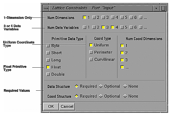
You can set any restrictions that make sense for your lattice port. This applies to both input and output ports which accept or produce lattices.
For example, Figure 2-3 shows the lattice definition for an input port called “Colormap.” The colormap lattice is a 1-D lattice with three or four floating point data variables (RGBA) per node. It has uniform coordinates and it must contain both data and coordinate values.
Table 2-1 shows how these specification are applied in the Lattice Constraints window.
Table 2-1. Colormap Lattice Constraints
Colormap Lattice Specs | Button Positions |
|---|---|
A 1-D lattice | Button #1 in the Num Dimensions field is ON |
Four data variables | Button #4 in the Num Data Variables field is ON |
Float data values | The Float button in the Primitive Data Type list is ON |
Lattice coordinates | All the buttons in the Coord Type list are ON |
Curvilinear coordinate variables per node | Buttons 1 through 3 in the Num Coord Dimensions list are ON |
Required values | The Required button is ON for both the Data Structure and Coord Structure fields |
Each field shown in the Lattice Constraints window defines a part of the lattice data type structure. The limits you set in this window should be consistent with the way the lattice is defined in the user function.
For more details on thelattice data type, see Chapter 3, “Using the Lattice Data Type.”
Click the radio buttons to activate the options. The light-colored, concave form indicates that the option is allowed.
In such cases, the Module Builder performs type coercion on the incoming data to convert it to the primitive type that the user function argument requires (see below).
| Note: The lattice primitive data types are C data types. If your user function is written in Fortran, select the C equivalents of the Fortran data types the user function expects (see Table 3-1 in Chapter 3). |
| Coord Type |
| |
| Num Coord Dimensions |
| |
| Data Structure and Coord Structure |
|
You can use the Data Optional/Coords Optional setting to allow the module to accept a lattice that has coordinate values but no data values. This lets you describe the geometry of a shape, such as a sphere or a pyramid mesh by using coordinate values only. You can then feed in a lattice containing data values only that show, for example, the variation in stress levels over the pyramid surface.
If you are working with lattice data and coordinate arrays, you can use the automatic type coercion facility. You can write a module's user function to operate on a single data type, such as a float, but allow the module to accept any primitive type as input on a specific port. The Module Builder then generates code to coerce data on that input port from its native primitive type to the primitive type required by the function argument to which the port is connected.
The Module Builder applies its coercion rules automatically during port and argument specification, based on the selections made in the Lattice Constraints window and the function arguments.
At run-time, the data is converted into the desired type, copied into memory, then passed to the computational function. Explorer assumes a 32-bit word length. The coercion proceeds as a series of individual coercions. Figure 2-4 shows the traversal path and the coercion pairs.
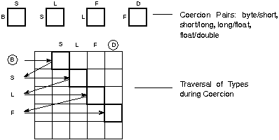
The C language process is:
D ⇒ F ⇒ I ⇒ SI ⇒ B, or double to float to int to short int to byte.
The Fortran language process is:
double precision ⇒ real ⇒ integer ⇒ integer*2 ⇒ character*1.
Out-of-range data is clipped to the acceptable range. Such coercions as
B ⇒ SI ⇒ I ⇒ F ⇒ D cause no loss of precision.
The following paragraphs describe the coercion process:
| Double to Float |
| |
| Float to Int | Float to Int coercion clips to the range of signed 32-bit integers, using the integer representation of the host computer and rounded to the nearest representable integer. | |
| Int to Short Int | The short int type stores integers between 0 and 65535. The translation maps [0,65535] to [0,65535] and clips integers outside the range to 0 or 65535. | |
| Short Int to Byte |
|
| Note: This feature makes module writing and integration much easier for the module writer, but it also requires time and a great deal of memory on the part of Explorer. It may be more efficient to write a module so that it accepts the correct data type without any coercion. This way, you will avoid the considerable “memory bloat” that is the cost of coercion. |
You can use the cxPyramid data type in a variety of ways. Some pyramids are built with every layer specified, and others are constructed in compressed form, with reference made to a standard structure in a pyramid dictionary for the compressed layers. The Pyramid Constraints window (see Figure 2-5) lets you specify whether the port can accept compressed or uncompressed pyramids and also establishes the level at which compression can take place.
For details on puramid compression, see Chapter 4, “Using the Pyramid Data Type.”
Click on the radio buttons to make your selections.
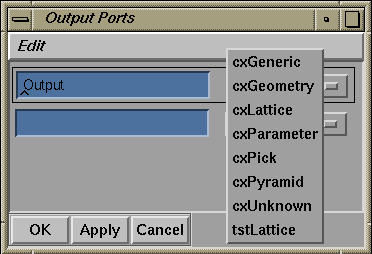
Figure 2-5 shows these default settings for pyramid constraints:
The pyramid must have four layers of lattices with connectivity information, that is three sets of lattice data and connections, and the base lattice.
The base lattice, which is the 0th-level lattice, is required.
The port can accept pyramids in all three compression modes, that is, uncompressed pyramids and compressed pyramids containing a variety of elements.
The port can accept pyramids that have been compressed at the third level. That is, compressed pyramids must be 3-D structures.
To display the Output Ports window (see Figure 2-6), click the Output Ports button on the Module Builder main window. The Map Editor uses the output port definition to decide whether a legal connection can be made between it and a given input port on another module.
The Output Ports window resembles the Input Ports window, except that it has only two fields, the port name and the data type.
For more details on the Geomerty data type, see Chapter 5, “Using the Geometry Data Type.”
The example in Figure 2-6 shows one output port with the port name “Output”. The data type it produces is cxGeometry, this meaning that the output port must be connected to an input port that accepts geometry data.
If you are creating an output port that produces a lattice, you set the data type to be cxLattice and the Lattice Constraints window appears again. Set the constraints for the output lattice exactly as you would those for the input lattice.
The Output Ports window does not require you to set the status flag because output ports are optional by definition; the module's firing pattern depends on the state of the input ports, not the output ports. A module that has the correct connections and data on its input ports will fire whether or not any output ports are wired.
You can write a smart module, that is, one that can track whether its outputs are wired and block certain computations if they are not connected. For example, the Render module has a camera output port for which data is calculated and output only if the port is wired.
You can code module with two output ports to check which output is wired and compute the data for only that one.You can then write a hook function for “connect output” and call the API function cxFireASAP from that hook function so that when you wire up the previously unwired output, the module will fire and send the new data downstream.
For more details on hook functions see Chapter 9, “Advanced Module Writing”.
When you define the function arguments, you are specifying the interface between the module itself, defined here as the Module Control Wrapper (MCW), and the user function. The Module Builder uses this information to generate bridging code, which takes the form of the Module Data Wrapper (MDW). This is the module's internal interface.
You use the Build Options menu to specify whether or not you want the Module Builder to write the MDW for you (see “Using the Build Menu.”)
You can take control of the interface and write your own interface code, in which case you do not need an MDW. If you write your own bridging code, you need not define the function arguments. Simply leave the Func Args and Connections windows blank.
For more details on writing wrapperless modules see Chapter 9, “Advanced Module Writing.”
You must enter the function name in the Func Name slot in this window (see Figure 2-7 and Figure 2-8) even if the module has no MDW; otherwise, you will get an error message telling you that the user function name is missing.
The Module Builder requires you to list each function argument and its correct type and referencing style so that the MDW can be written correctly. To display the Func Args window (see Figure 2-7), click the “Func Args” button on the Module Builder main window.
The examples in Figure 2-7 and Figure 2-8 show the argument lists for the VectorGen and AtomicSurf modules. The fields in the Func Args window are described below.
The Func Name is the name of the user function or subroutine. It is repeated at the bottom of the window, along with the complete list of arguments. The Module Builder uses this field to create a call to the function.
Type the name in the text type-in slot exactly as it appears in the user function file.
The Language button of the Function Args window allows you to select the language in which the user function or subroutine is written. The Module Builder uses this field to determine the calling conventions for the wrapper code (which is generated in C).
Select C, Fortran, or C++ from the Language pop-up menu.

The Arg Name section of the Function Args window lists the function argument names, entered in the correct calling sequence. The Module Builder uses this list to establish the calling sequence of arguments for the function when it creates the Module Data Wrapper (MDW).
Type the name of the first argument and press <Enter> to get a new slot.
Use the Edit menu to copy or reposition function arguments in the list.
Use OK or Apply to update the calling sequence when you have entered a new argument.
To remove an argument from the calling sequence, simply delete the name of the argument from the list.
You can enter up to 45 function arguments per function. Each argument must have a unique name. The Module Builder renames duplicate arguments.
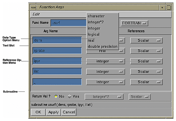
The Type section of the Function Args window lets you select a data type for each argument variable. These differ for C and Fortran.
Figure 2-7 shows the data type options menu for a C function. The menu is the same for C++ functions. Figure 2-8 shows the options for a Fortran subroutine.
Select one option from the menu for each argument.
Table 2-2 shows the relationship between the C and Fortran primitive data types that Explorer recognizes.
Table 2-2. Primitive Data Types in C and Fortran
C and C++ | Fortran |
|---|---|
char (byte) | character*(1) |
short | integer*2 |
int | integer |
long | integer |
int | logical |
float | real |
double | double precision |
pointer | integer |
cx* | integer |
In the C and C++ options menu, Explorer data types or subsidiary types (cx<DatatypeName>) are followed by an asterisk (*). They are automatically passed by reference because they are arrays written in C. In Fortran, you refer to the Explorer data types by using integers that contain a pointer to the C data structure. The C structures that are referenced can be manipulated through the Fortran API, but not directly in the syntax of the language. The pointers are uniformly treated as “opaque handles” that are passed around in integer variables.
The References section of the Function Args window lets you set the method whereby the argument variable is passed. Figure 2-7 shows the data type options menu for a C function. The menu is the same for C++ functions. Figure 2-8 shows the data type options menu for a Fortran function.
The choices are by value or reference in C or C++, by reference only in Fortran. Table 2-3 shows the choices for C, C++, and Fortran.
| Note: The term “references” is used here in the C sense, rather than the C++ sense, where it has a slightly different meaning. |
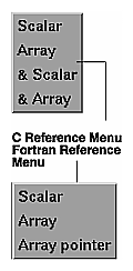
Table 2-3. Function Argument References
C and C++ | Fortran | Purpose |
|---|---|---|
Scalar | Scalar | Used for passing in a single value. Scalars are passed by value in C and C++ |
Array | Array | Used for passing in or modifying a data array. Expects multiple values. Arrays are passed by reference in C and C++. |
& Scalar | [a] | Used for passing a value out by means of the argument list. Passes a pointer to a scalar. |
& Array | Array Pointer | Used for passing out an array by passing a pointer to an array reference, such as an array allocated in the function. Also useful for returning a pointer to allocated storage. |
[a] Because Fortran always passes parameters by reference, there is only one option, Scalar, for passing Fortran scalar values. | ||
The choices in the Return Val? section of the Function Args window indicate whether the user function or subroutine returns a value. If it does, you must select a type and reference as you did for each argument. The return value can be used when you set up connections from the function arguments to the output ports (see “Connecting Arguments to Ports” below).
When you have entered and defined all the function arguments in their correct calling sequence, click OK to save the argument list and close the window.
The user function arguments, once defined, must be associated with the input and output ports so that incoming data goes to the correct function arguments for processing before being passed in turn to an output port.
To display the Connections window, click on the “Connections” button on the Module Builder main window. The Connections window displays graphically the links between inputs, function arguments, and outputs. When you first create a module, no connection wires are shown. The wires appear after you have used the mouse to make a link between an argument and a port.
Figure 2-9 shows the connections between the function arguments for VectorGen and its ports. There are two input ports, “Input” and “Scale Factor,” and one output port, “Output”. The function arguments are listed in the center column. The open port menu in the center of the screen is the connections menu for “Scale Factor,” which passe the parameter data type.
There are also three “pseudo” input ports listed under Input Ports. Please refer to “Using Pseudo Input Ports.”
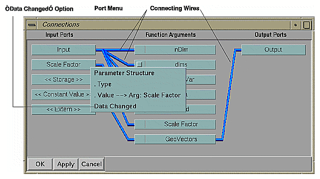
Each port has a connections menu that gives its data type structure and lists the constituent elements of the data type. The number of dots in front of each element name indicates how many levels below the top-level data structure you have penetrated.
For example, in Figure 2-9 it is clear from the menu that a link has been made between the Value element in the Parameter structure and the Scale Factor function argument. This means that any data value passed from an upstream module to the “Scale Factor” input port of VectorGen is sent in turn to the Scale Factor function argument. The Value element has one dot in front of it; it is one level below the Parameter structure and on a par with the Type element.
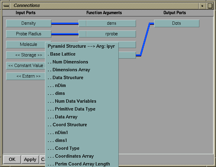
Lattice, pyramid, and pick data types have several substructures that can be wired to or from function arguments. Figure 2-10 shows the Connections window for AtomicSurf, which has an input port, “Molecule,” that accepts the pyramid data type. Part of the connections menu for this port is shown. As you can see, Pyramid Structure, which includes the entire contents of the data type, is connected to the function argument ipyr.
The other items on the menu are the substructures of the pyramid data type. They include:
individual scalars, such as the number of variables per node (Num Data Variables)
arrays such as the dims vector (Num Dimensions) and the data and coordinate arrays (Data Array and Coord Array)
C data and coordinate structures, such as Data Structure and Coord Structure, of which the scalars and arrays are constituents
You can write function arguments that accept data from any one of these substructure if you wish.
You can use a pointer to the C structure to pass a complete Explorer data type directly to a function argument if the user function is written in Fortran or the function argument is broken into smaller elements of the data type.
The physical mechanism of wiring ports and functions together and disconnecting them again is exactly the same as that used in the Map Editor. Click on an input port with the right mouse button, select the element to be wired, and then click on the function argument (or output port). The Connections menu for function arguments has only one item, “Select.” To break a connection, simply reverse the process.
The “- - >” icons in the connections menus show which elements of an input or output port are associated with each other or with function arguments.
You can make only one connection to a given function argument from an input port, and only one connection from a given function argument to an output port.; however, you can make several connections from an input port or to an output port. For example, the “Input” input port in Figure 2-9 has four connections, one to each of four function arguments.
All function arguments must have a connection to either an input or an output port, but all ports do not necessarily have to be connected.
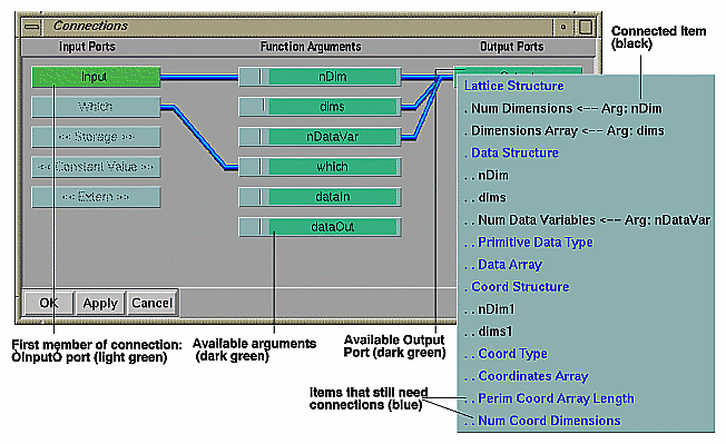
Figure 2-11 shows how connection options are highlighted in the Connections window. There are two kinds of highlighting:
When you select a port menu item or function argument as the first member of a connection, the selected item turns light green, and the available options from which you can select the second member turn darker green.
Unavailable items are grayed out (in Figure 2-11, these are the remaining input ports).
When an output port lacks a connection required for the integrity of the data type on the port, the connections menu lists the relevant item in blue. When you first open the Connections window, no connections exist and the entire list of data structures is blue. As connections to the output port are made, the connected structure is listed in black.
This color coding helps you to see whether the output port will receive all the data it needs to construct a complete data type.
In many cases, you can connect the top-level data structure on the input port directly to the top-level data structure on the output port in order to pass default values. For example, in a module that accepts a lattice on an input port and outputs a lattice on an output port, you can connect the cxLattice structure at the top of the input port menu to the cxLattice structure at the top of the output port menu.
In this way, all data that is not affected by a function argument will be passed by default from the input port to the output port. The members of cxLattice that were operated on by function arguments will acquire new data that is passed in turn to the output port to replace the old data.
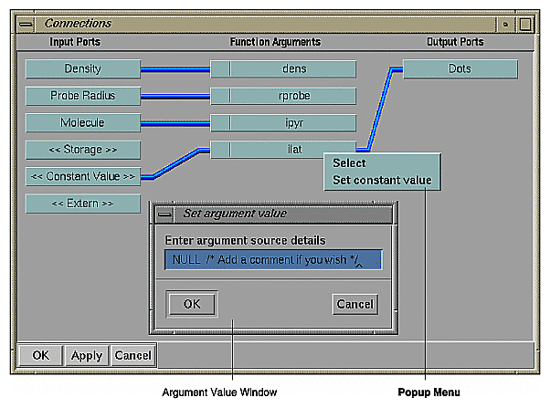
At the bottom of the Input Ports list are the three so-called “pseudo” input ports, <<Storage>>, <<Constant Value>>, and <<Extern>> (see Figure 2-12). They cannot be wired directly to output ports, unlike the regular input ports. However, you can connect them to function arguments to do these things:
Once you have wired the <<Storage>> or <<Constant Value>> ports to a function argument, the argument's connection menu acquires a second item. To se the argument click on it after the connection has been made.
The second item, “Set Storage” or “Set Constant Value”, when selected, invokes the “Set argument value” window. Figure 2-12 shows the connection between the <<Constant Value>> input port and the GeoVectors function argument in VectorGen, the GeoVectors connections menu, and the value set (NULL, which is the default). See “Allocating Storage Space” for more information about temporary storage.
You can enter any legal C or Fortran expression in the text slot, including references to library or user-supplied routines that can be resolved at link time. It is a good idea to comment on your entries for future reference.
<<Extern>> can be wired to only a function argument whose variable name refers to the name of another function or subroutine. This function must be in a module source file and referenced in the User Function File slot in the Module Builder main window (see Figure 2-1 ).
to reference numerical analysis routines. For example, you can specify the name of a routine that executes a particular action, such as a convergence test. The name of the function argument should be identical to the function name. The function argument is then the function returning a long scalar.
in an integrator module, to pass in either a function to be integrated, or a derivative function.
Here is an example of how to use <<Extern>>. Suppose you have a function named calcDerivative and you want the user function to use this derivative calculating function in its global optimization calculation. You would need to:
set a function argument name to calcDerivative
wire <<Extern>> to the calcDerivative function argument
treat that function argument as a function or subroutine in the user function.
These are the basic rules to follow when connecting ports and arguments:
The mapping to an output port must describe the contents of the output data structure fully. Every element in an output port should have a source, either a function argument or an input port; otherwise the Module Data Wrapper may not have enough information to build the data set and errors will appear (not immediately, where they can be picked up, but later, and apparently mysteriously).
On port menus, you can wire to the data type structure itself or to all its component elements. For example, instead of wiring to Pyramid Structure in Figure 2-10, you can wire to all the substructures listed as separate elements. Similarly, you can wire to Data Structure or you can wire to Num Data Variables, Primitive Data Type, and Data Array, which are subelements of the Data Structure component.
Wire input ports to function arguments and/or output ports. Ports can have multiple connections (one to each part of the data structure on the port menu). Function arguments can have only one input and only one output (but need not have any outputs).
If you make more than one connection to a function argument or a port menu element, you may duplicate and/or overwrite data as it is passed, causing errors. In particular, if you wire more than one connection to an output port element, you run the risk of leaking memory.
Every function argument must be connected to an input port, a pseudo input port, or an output port. You can leave only one unconnected if you do not intend to use it.
You can wire an input lattice data type to an output data type, but the values of nDim (Num Dimensions) and dims (Dimensions Array) cannot be changed. This is a mistake easily made because the data and coordinate substructures (cxData and cxCoord) each have a copy of these values.
At the bottom of each connections menu is the Data Changed item (see Figure 2-9).You can use it to record whether the module received new data on that particular port during the most recent firing. Depending on the answer, the user function may then act to collect new data from the port, or ignore the old data. Data Changed returns a long integer with the value 0 (to indicate old data) or 1 (to indicate that new data has arrived on the port).
You can wire Data Changed to any scalar function argument.
Arrays listed as function arguments in the Connections window have Copy buttons that let you choose between copying pointers to arrays and the arrays themselves, depending on whether data is to be overwritten or not. The Copy button appears at the left side of the array function argument. When you click a Copy button, it is lit and the word “Copy” is displayed (see Figure 2-13).
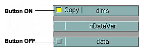
This copy facility is important if you intend to modify the contents of an argument whose original values come from an input port. Since data from an input port resides in shared memory, it cannot be written into without polluting the data space of other modules and causing a module in the map to fail.
When the Copy button is ON, it tells the Module Builder to make a working copy of the array so that you can modify it. This is useful even if you intend to use it only as a temporary working space, without writing it to an output port.
For example, in a module that manipulates the grid data of a lattice without changing the coordinates, data will be overwritten; therefore, the Copy button should be turned ON. If the Copy button is OFF, a pointer to the array is passed.
Scalars are always copied before being passed to the user function.
You can use the <<Storage>> pseudo input port to allocate temporary storage space in cases where the data is to be modified. The space can be used as follows:
Two API routines are useful for computing the size of arrays for wiring to the storage allocator (see the IRIS Explorer Reference Pages for details):
cxDimsProd computes the total number of data variables in a lattice.
cxDimsSum computes the length of the perimeter coordinate vector for a lattice.
After the user function has been invoked, the allocated storage is freed. The Module Data Wrapper automatically frees working space that has been held temporarily by the user function. The Module Builder uses reference counting to maintain temporaries assigned to output ports as part of the output port list.
You must free any temporaries that you create inside the user function.
You can use the Prototypes menu in the Module Builder main window (see Figure 2-14) to create a prototype user function and a help file for your new module.
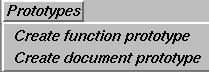
The Module Builder will create a user function prototype for you if you have not already written it, or do not have existing code for it. You must already have named the function and laid out the calling sequence of the function arguments in the Func Args window. The Module Builder uses this information to write a stub function that is the user function as described, but without any action.
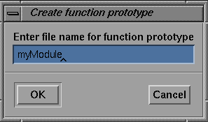
When you select “Create function prototype” from the Prototypes menu, a window appears, in which you enter the name you want for the new user function (see Figure 2-15). The file is created in your working subdirectory, along with the other module files. If a file with the name you have selected already exists, the prototype file is renamed <filename>.user.
This example shows a basic prototype for a user function MyModule.c. The module has lattice input and output ports and parameter input ports. The user function is written in C and has 12 function arguments.
#include <cx/cxLattice.api.h>
#include <cx/cxParameter.api.h>

#ifdef __cplusplus
 extern “C” {
#endif

 void MyModulec (
 long    dim,
 long    dim,
 long    dim,
 long    *dims,
 long 				nDataVar,
 double 				*dataArray,
 long 				nCoordVar,
 float 				*coordArray,
 long 				*nDimOut,
 long 				*dimsOut,
 double 				*dataOut,
 float 				*coordOut );

#ifdef __cplusplus
}
#endif

/* ------------------------------------------- */
/* ------------------------------------------- */

 void MyModulec (
 long         Idim,
 long         Jdim,
 long         Kdim,
 long         *dims,
 long         nDataVar,
 double       *dataArray,
 long         nCoordVar,
 float        *coordArray,
 long         *nDimOut,
 long         *dimsOut,
 double       *dataOut,
 float        *coordOut )
{
}
|
Once you have the prototype file, you can open it and finish writing the user function at your leisure. If you create the prototype file before you have defined the function in the Module Builder, the file will not contain the function arguments.
You can generate a function prototype for each hook function you want to write for a module. To create the hook function, use the “Hook Funcs” option on the Build menu (for details, refer to “Hook Functions.” Then select “Create function prototype” from the Prototypes menu to create the hook function prototypes.
Here are examples of the two types of hook function prototype in Fortran.
C Hook function for Explorer module actions. /*Remove hook /*
      SUBROUTINE FREMOVE()
      print *,'Remove hook function called.'

      RETURN
      END

C Hook function for Explorer module actions. /* Connection /*
      SUBROUTINE FCONNIN( PORTNAME, LINKTAG)
      CHARACTER*(*) PORTNAME
      *INTEGER LINKTAG
      print *,'Connect input hook function called: ',
     1*PORTNAME, LINKTAG

      RETURN
      END
|
If you want the Module Builder to create a help file template for you, select “Create document prototype” from the Prototypes menu on the Module. The help file is saved in your working directory with the name <modulename>.doc.
A skeleton file contains the port names, data types, and other variables that you have specified during module building. You should add any descriptive information you want users to read when they invoke help for your module. This information should include a description of the module's algorithm, ports, known problems or limitations, and related modules. Be careful not to disturb any line beginning with %%.
This example shows what the prototype help file for MyModule.c, called MyModule.doc, would look like.
MyModule %%------------ DESCRIPTION ------------ <Replace this with your module description> %%------------ INPUTS ------------ %PORT Input 1-D %TYPE Lattice %CONSTRAINT 1-D %CONSTRAINT curvilinear <Describe the purpose of the port here> %PORT I dimension %TYPE Parameter <Describe the purpose of the port here> %PORT J dimension %TYPE Parameter <Describe the purpose of the port here> %PORT K dimension %TYPE Parameter <Describe the purpose of the port here> %%------------ WIDGETS ------------ %%------------ OUTPUTS ------------ %PORT Output 3-D %TYPE Lattice %CONSTRAINT 3-D %CONSTRAINT curvilinear <Describe the purpose of the port here> %%------------ PROBLEMS ------------ <Describe any known problems/limitations here> %%------------ SEEALSO ------------ <List associated or related modules here> |
If you are modifying an existing module and changing some aspect of its control panel (such as using different widgets or new ports), select “Update document” from the Build Options menu (see Figure 2-16) to update the existing <modulename >.doc file and preserve any existing annotation.
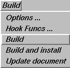
The Build menu (see Figure 2-16) provides a way to set some defaults for the module and to choose the directory in which modules will be built and installed: in your working directory, or in another directory of your choice. All the menu options except “Hook Functions” are discussed below. Hook functions are discussed in “Hook Functions.”
You can set a number of options in the Build Options menu (see Figure 2-17):
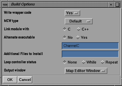
| Write wrapper code |
| |
| MCW type | Lets you select the type of Module Control Wrapper (MCW) for linking. Most modules link against the default MCW, but a few manipulate windows in the X Window System independently of the Explorer graphical user interface (see examples in “Working with Module Wrappers”). These modules should be linked against the X-MCW. | |
| Link module with | ||
| Alternate executable |
| |
| Additional Files to Install |
| |
| Loop controller status |
| |
| Output window |
|
The last three options on the Build menu do not have any menu choices. The “Build” and “Build and install” options simply initiate the compilation and installation process on the module. The “Update document” option tries to update the module modulename.mres file and gives you an error message in the shell window if it fails.
“Build” builds the module in the current working directory.
“Build and install” installs a module in /usr/explorer/module by default, irrespective of where it is built. If you want a module to reside in a directory other than /usr/explorer/module, you need to set the EXPLORERUSERHOME environment variable before you start the Module Builder. This variable is described in “Configuring the Build Environment.”
Use the “Build and install” command in the Module Builder instead of “Build.” It will install your completed module in the correct directory.
Some modules, particularly modules that contain an interpreter that reads a script file, but perhaps other modules as well, have auxiliary files that need to be installed when the module is installed. For instance, LatFunction-based modules have a script file (named in the “Program File” widget) that should be installed to go along with the module.
This is automatically handled by the interpreter option when you specify an alternate executable, but you can use the Build Options menu to install other files as well if you wish (see “Selecting Build Options.”)
The “Update document” option updates both the modulename.mres file and the document help file (.doc). You must have write permission on the module's modulename.mres file to do this.
The document file is overwritten and the original .doc file is saved as a .bak file. if you have information in the old file that you want retained in the new file, you must edit the new .doc file accordingly. These are ASCII files, so this is easily done.
The modulename.mres file is overwritten without any backup file being saved.
The Module Builder handles the details of the module building and installation environment, but it does not handle creation of data types. These you must make yourself (see Chapter 8, “Creating User-defined Data Types.”) When you do so, you may want to designate a different installation directory for your new data types and modules.
You must define one very important environment variable to indicate to the Module Builder where new modules and type files are to be installed:
Typically, the value of this variable would be /usr/local/explorer or perhaps $HOME/explorer. For example, in the C-shell you would type this command:
setenv EXPLORERUSERHOME /usr/local/explorer
When modules and types are built, the generated Makefile installs a number of items under EXPLORERUSERHOME, creating subdirectories as necessary. This is the directory structure created under $EXPLORERUSERHOME: $EXPLORERUSERHOME/
A few environment variables control alternatives when modules are built and installed. They need not have any particular value, and they take effect:
only if defined
after you rebuild the Makefile (see below)
The variables are:
| CXBUILDSHARED |
| |
| CXINSTALLSYMBOLIC |
| |
| CXINSTALLSTRIPPED | | |
| DEBUG | Modules will be compiled with the debug option, -g. Explorer modules are compiled by default with the compiler's optimizer option, -O. You must set the DEBUG option before you make the module Makefile if you want to be able to debug your module. For more information, see “Debugging a Module.” |
When you issue the make install command in a directory used for building modules or data types, the files are created and installed in the directories according to the environment variables you have set. If you ever change the value of these variables, you must recreate the Makefile in your directory to reflect the new value.
You can do this with the command:
make Makefile |
If you do not already have a Makefile, you must use the command:
cxmkmf |
This command makes you a new Makefile, which you can use to recreate your modules and type-related files.
Modules built in a directory are listed in a special file named MODULES; the Module Builder creates this file for you. New data types must be listed in a file named TYPES, which you must create by hand, since there is no mechanism for listing new data types automatically.
The TYPES file must contain the names of the data type files to be processed in the current directory, but without the .t suffix. For example, if you have data type files named NewType.t and MyType.t, then you must create a TYPES file that contains the files: For more on .t files, see Chapter 8, “Creating User-defined Data Types.”
NewType MyType |
Both the MODULES and the TYPES files must be present before you run cxmkmf. Then cxmkmf creates the Makefile commands required to build and install code properly for these data types.
For more information on Makefiles, read Appendix A, “Using Makefiles.”
To compile a module with the -g option for debugging purposes, set the DEBUG environment variable before you issue the cxmkmf command.
When you are ready to make the module, type these commands:
setenv DEBUG 1 cxmkmf make MyModule |
You can then debug your module. To do this, start Explorer with the module in it:
explorer MyModule |
In a separate shell window, bring up your favorite debugger. Some examples are:
dbx -P MyModule |
or
edge -P MyModule |
or
cbd |
and attach it to the running process.
To profile a module, you must build the module with the profiling option turned on. To get profiling turned on for the module executable, you must set the link option -p. You can do this by:
typing -p in the Libraries text slot in the Module Builder main window (see Figure 2-1)
adding the line
LOCAL_LD FLAGS = -p
to your user-supplied Makefile. This is the better way to do it.
When you start Explorer, make sure that the module is installed and that you run the profiled executable for the module.
You cannot profile a module that uses shared libraries. If your module usually does, for example, if it uses Inventor or X Windows, bring up the Module Builder, add -lc in the Libraries line, and resave the modulename.mres file. The Module Builder will build the module with unshared libraries.
Then type:
prof modulename mon.out |
The profiling output is saved into the file mon.out in your current directory. For more information on the profiling command, refer to the UNIX man page for prof(1).
This is a brief summary of the steps you must take if you want to profile an Explorer module using the pixie command. It is not an exhaustive description. For more information, refer to the UNIX man page for pixie(1).
You may want to profile more than one module together to determine whether the transfer of data between them is efficient. For example, the first module may fire many more times than is necessary to generate the requisite data for the downstream module. Carry out the following steps on all modules to be profiled:
Run pixie on each module. This creates two files, modulename.pixie and modulename.Addrs. If the module uses shared libraries, it also creates the files sharedlibname.pixie and sharedlibname.Addrs.
Save the original module somewhere safe with a different name. For example, use the suffix .save.
Move all *.pixie and *.Addrs files to a central directory and cd to that directory.
Copy each modulename.pixie module to the original module.
Run Explorer to execute each module normally. This creates a file called modulename.Counts.
Replace each modulename.pixie with the original module.
Make sure you are in the directory containing the *.Addrs and *.Counts files, then run
prof -pixie modulename
The biggest drawback to pixie is that it does not support shared libraries. If you profile more than one module that uses shared libraries, the results are written to the same .Counts file and you get inconsistent or garbled results.
Here are user functions for two simple modules, coded in C and in Fortran. The first one is a simple pass-through module, and the second is a channel-select module. The source code for these modules is in /usr/explorer/src/ModuleBuilder/C/ * and /usr/explorer/src/ModuleBuilder/Fortran/ *.
This module copies a given input to the output. The user merely modifies the assignment statement in the loop to perform an operation on the data.
#include <cx/DataAccess.h>
#include <cx/DataTypes.h>
#include <cx/cxLattice.api.h>

void pass  (
    cxLattice *inlat,
    cxLattice  **outlat )
{
    float          *inData, *outData;
    long            nDim, *dims, nDV, nCD;
    long            num_pts, i, hasData, hasCoord;
    cxData         *Data;
    cxPrimType      ptype;
    cxCoordType     ctype;

    *outlat = cxLatDup(inlat, 1, 1);
    cxLatPtrGet(inlat, &Data, &inData, NULL, NULL);
    cxLatPtrGet(*outlat, NULL, &outData, NULL, NULL);
    cxLatDescGet(inlat, &nDim, &dims, &hasData, &nDV,
        &ptype, &hasCoord, &nCD, &ctype);

    num_pts = cxDimsProd(nDim, dims, nDV);
    for (i = 0; i < num_pts; i++) {
        *inData++ = *outData++;
    }
}
|
      subroutine pass(inlat,outlat)
      implicit none

      integer inlat, outlat, cxLatDup, cxDimsProd
      real inData(1),outData(1)
      integer nDim,dims(1),nDV,nCD
      integer num_pts,i,hasData,hasCoord
      integer Dataptr,ptype,ctype
      pointer (PinData,inData)
      pointer (PoutData,outData)
      pointer (pdims,dims)

      outlat = cxLatDup(inlat,1,1)
      call cxLatPtrGet(inlat,DataPtr,PinData,ctype,ptype)
      call cxLatPtrGet(outlat,i,PoutData,ctype,ptype)
      call cxLatDescGet(inlat,nDim,pdims,hasData,nDV,
     1    ptype,hasCoord,nCD,ctype)

      num_pts = cxDimsProd(nDim,dims,nDV)
      do i=1,num_pts
         inData(i) = outData(i)
      end do

      return
      end
|
This module selects a channel.
/* sample module that does a channel select */
#include <cx/Typedefs.h>
#include <cx/DataTypes.h>
#include <cx/DataAccess.h>
#include <cx/UI.h>
channel(long which, cxLattice *inLat, cxLattice **outLat)
{
  long xLo,xHi,i,j,k,nData,dataLen,w;
  long nDim,nDataVar,hasData,hasCoord,nCoordVar,*dims;
  cxCoord *coord;
  cxPrimType primType;
  cxCoordType coordtype;
  cxData *data;
  char *oldData, *dataArray;

/* Get all the information about the input lattice */

  cxLatDescGet(inLat,&nDim,&dims,&hasData,&nDataVar,&primType,               &hasCoord,&nCoordVar,&coordtype);
  cxLatPtrGet(inLat,&data,&oldData,&coord,NULL);

/* reset the range of the slider based on the number of input data variables */

  xLo = 1;
  xHi = nDataVar;
  cxInWdgtLongMinMaxSet( “Which Data”, xLo, xHi);

/* reset range of widget if off-scale */

  w = which;
  if(w > xHi){
    w = xHi;
    cxInWdgtLongSet(“Which Data”,xHi);
  }
  if(w < xLo){
    w = xLo;
    cxInWdgtLongSet(“Which Data”,xLo);
  }

/* Make a new lattice of the correct size */

  w -= 1;
  nDataVar = 1;
  *outLat = cxLatDataNew(nDim,dims,nDataVar,primType);

/* move the coord pointer from the old lattice to the new lattice */

  cxLatPtrSet(*outLat,NULL,NULL,coord,NULL);

/* get the information about the new data array */

  cxLatPtrGet(*outLat,NULL,&dataArray,NULL,NULL);
  nData = cxDimsProd(nDim,dims,nDataVar);
  dataLen = cxDataPrimSize(data);

/* copy the data from the old array to the new array */

  oldData += dataLen * w;
  for(i=0;i<nData;i++){
    bcopy(oldData,dataArray,dataLen);
    oldData += dataLen * xHi;
    dataArray += dataLen;
  }

/* all done */

}
|
      subroutine channel(which,inLat,outLat)
      implicit none
      integer which,inLat,outLat
      include '/usr/explorer/include/cx/DataAccess.inc'
      integer nDim,dims(1),hasData,nDataVar,primType
      integer hasCoord,nCoordVar,coordType,w,i,j,k,l,p0
      integer nData,dataLen,data,xHi
      real coord(1)
      character *1 oldData(1),dataArray(1)
      pointer (pdims,dims)
      pointer (pdata,data)
      pointer (pcoord,coord)
      pointer (poldData,oldData)
      pointer (pdataArray,dataArray)
      p0 = 0
      call cxLatDescGet(inLat,nDim,pdims,hasData,nDataVar,
     1     primType,hasCoord,nCoordVar,coordType)
      call cxLatPtrGet(inLat,pdata,poldData,pcoord,p0)
      p0 = 0
      w = min(max(1,which),nDataVar)
      call cxInWdgtLongMinMaxSet(“Which Data”,1,nDataVar)
      call cxInWdgtLongSet(“Which Data”,w)
      w = w - 1
      xHi = nDataVar
      nDataVar = 1
      outLat = cxLatDataNew(nDim,dims,nDataVar,primType)
      call cxLatPtrSet(outLat,p0,p0,pcoord,p0)
      call cxLatPtrGet(outLat,p0,pdataArray,p0,p0)
      nData = cxDimsProd(nDim,dims,nDataVar)
      dataLen = cxDataPrimSize(pdata)
      do i=1,nData
         k = dataLen*(i-1)
         l = dataLen*((i-1)*xHi+w)
         do j=1,dataLen
            dataArray(k+j) = oldData(l+j)
         end do
      end do
      return
      end
|
[2] cxGeneric is a special case, a data type which can be wired to any other data type. It is described in Chapter 7.