This chapter defines the lattice data type and how it is used in the Explorer environment. It describes the forms that lattices can take in one, two, and three dimensions and gives examples of how to create them.
The API (Application Programming Interface) routines are listed and examples of user function code for writing modules that manipulate lattices are included.
The Explorer lattice data type, cxLattice, contains all the information Explorer requires for creating arrays. An array is a regular, structured matrix of points, which can be 1-D or multidimensional. Because it is extremely versatile, you can use the cxLattice data structure to represent a wide variety of array data. For example, some modules may accept a cxLattice with any number of dimensions, containing any number of data values, of any type. Other modules may accept only 1-D lattices in byte format. In general, the form of the array data you plan to feed into a module will determine how narrowly you define the lattice specifications on the input port in the Module Builder.
The Explorer lattice data structure has two arrays, one holds data values and one holds node coordinates. A node is a point in a lattice defined by a unique coordinate or set of coordinates in Cartesian space, usually indicating the position of the data value (or values). The data and coordinate arrays are optional, however. You can create a lattice with an empty data structure, and node coordinates only, or one with data values and no coordinate values.
The two array structures in cxLattice are cxData and cxCoord. The data and coordinate arrays are defined in separate variables because:
The Cartesian space in which the lattice exists may be irregular, for example, in a finite difference-based simulation program. Such programs may require complicated physical mappings even though the data is straightforward.
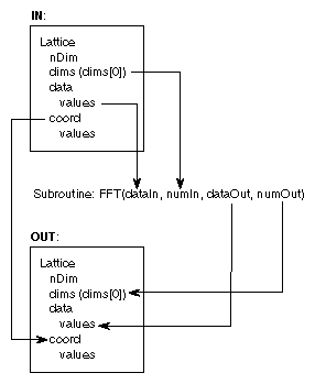
Two different lattices, such as an input and an output lattice, can share the same data or coordinate array, thereby saving memory. For example, the lattices may have different data but use the same coordinate values.
Figure 3-1 illustrates the principle of sharing array values. The lattices on the module input port and on the module output port use the same coordinate values, which are passed directly from input to output, but the data values change from input to output as they are processed by the user function.
The cxLattice data type is one of the root data types, which means it can be placed on module ports and will pass data into and out of modules. It has three main parts, or subsidiary data structures:
 | Note: The dimensions of cxData and cxCoord are set by the nDim and dims variables. Both arrays must have the same value for nDim and dims. |
This is the type definition for cxLattice:
shared root typedef struct {
     long                *nDim        “Num Dimensions”;
     long*               *dims[nDim]  ”Dimensions Array”;
     cxData(nDim,dims)   *data        “Data Structure”;
     cxCoord cDim, dims) *coord       “Coord Structure”;
} cxLattice;
|
The type definitions for cxData and cxCoord are given in the next few pages. Figure 3-2 shows a schematic representation of cxLattice.
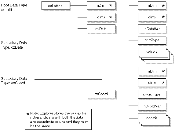
The dimension variables in the cxLattice data type are:
The nDim variable indicates the number of dimensions of the lattice. In curvilinear lattices, it indicates the number of parameter variables. The dims array specifies the number of nodes in each dimension, that is, the number of data values in each dimension.
In Figure 3-2, nDim and dims are stored with both cxData and cxCoord; these values however, must be consistent throughout the cxLattice structure; otherwise, you may get some bizarre results. For example, if you define nDim as 3 and dims as [10,6,6] in cxData, you must also define them as 3 and [10,6,6] in cxCoord.
Data values go into the cxData type, which contains the value or values stored at each node of the lattice. Its elements include:
the dimension variables, nDim and dims
the number of data variables per node, nDataVar
the type of primitive variable that can be used for data values, primType. There are five options (see Table 3-1).
the array of data values
This is the data type definition for cxData:
shared typedef struct { /* Explorer Lattice's Data array */
 long       nDim;
 long       dims[nDim];
 long       nDataVar     “Num Data Variables”;
 cxPrimType primType     “Primitive Data Type”;
 switch     primType) {
    case cx_prim_byte:
       char  values[nDataVar, dims] “Data Array”;
    case cx_prim_short:
       short values[nDataVar, dims] “Data Array”;
    case cx_prim_long:
       long values[nDataVar, dims] “Data Array”;
 case cx_prim_float:
       float values[nDataVar, dims] “Data Array”;
  case cx_prim_double:
        double values[nDataVar, dims “Data Array”;
    } d;
} cxData(nDim, dims);
typedef enum {
  cx_prim_byte,
  cx_prim_short,
  cx_prim_long,
  cx_prim_float,
    cx_prim_double
  cxPrimType;
|
The Cartesian coordinate values that define the position of the lattice nodes go into the cxCoord data type. These values map the lattice data to Cartesian space. Its elements include:
This is the data type definition for cxCoord:
shared typedef struct { /* Explorer Lattice's Coordinate array */
  long         nDim;
  long         dims[nDim];
  cxCoordType   coordType             “Coord Type”;
  switch       coordType) {
    case         cx_coord_uniform:
       float        bBox[2, nDim]     “Coordinates Array”;
    case         ex_coord_perimeter:
         long       sumCoord          “Perim Coord Array Length”;
       float        perimCoord[sumCoord]  “Coordinates Array”;
    case         cx_coord_curvilinear:
        long        nCoordVar          “Num Coord Dimensions”;
          float     values[nCoordVar, dims] “Coordinates Array”;
  }           c;
} cxCoord(nDim, dims);
|
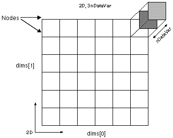
Figure 3-3 shows the relationship of some lattice variables. This example depicts a 2-D lattice with seven nodes in each dimension and three data variables per node. Thus, nDim = 2, dims[0] = 7 (x direction), dims[1] = 7 (y direction), and nDataVar = 3.
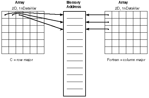
The lattice and coordinate data values are stored separately and in different formats. Figure 3-4 shows how data from lattices in C and Fortran formats is stored in computer memory. The formats used by each data and coordinate lattice type in cxLattice format are described below.
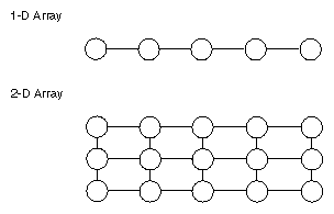
Lattice data is located at the coordinate nodes. In a 1-D array, or vector, each node in the array has two neighbors (except the end points, which each have only one), as shown in Figure 3-5. In two dimensions, each internal node has four neighbors. A node internal to a 3-D array has six neighbors. An internal node in an n-D array has 2*n neighbors. This regular structure is the computational space of the array.
Lattice data is stored in the Fortran convention, using a column-major layout, in which the I direction of the array varies the fastest (see Figure 3-6). For all lattice types, the I direction corresponds to the X direction. Similarly, J corresponds to Y, and K to Z.
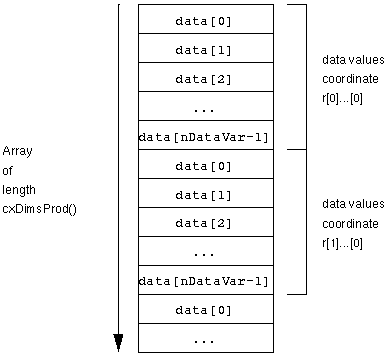
If a lattice has several data values at each node (that is, if nDataVar > 1), then the data is stored in interleaved format. In a color image, for example, the interleaving of RGB data looks like this:
R(node 1) G(node 1) B(node 1) R(node 2) G(node 2) B(node 2) R(node 3) G(node 3) B(node 3)... |
To locate a particular node within an array, you use array indexing. For example, the node located at (i,j,k) is:
Array[k][j][i] in C Array(i,j,k) in Fortran |
You can compute the number of nodes in a lattice by calling the subroutine cxDimsProd. You can also use this function to compute the total number of data variables. See the IRIS Explorer Reference Pages for details on the API subroutines.
The primitive data type is defined in terms of C values in the lattice data type. If you are programming in Fortran, choose the C primitive that is equivalent to the Fortran variable that your subroutine expects. Table 3-1 lists the equivalences between the two.
Table 3-1. Lattice Primitive Types
C Data Types | Fortran Equivalents |
|---|---|
integer (integer*4) | |
double precision (real*8) |
Coordinates are always stored in single-precision floating point (float) format. The lattice data type allows for three types of coordinate mapping to physical space: uniform, perimeter, and curvilinear. The interleaving of the coordinate storage varies from type to type. Each type is described in detail below.
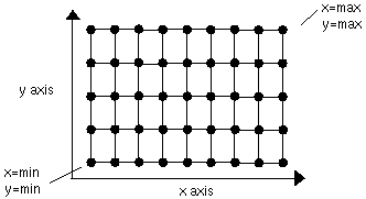
A lattice with uniform coordinates has a uniform cell size throughout (see Figure 3-7). Most generated data is in this format.
The data structure for a uniform lattice is:
struct {
    float    *bBox; /* An array of length [2, ndim]*/
} cx_coord_uniform;
|
The coordinate values are stored in row-major format, in the C convention:

Explorer uses a bounding box to set the size and aspect ratio of lattice coordinates. Bounding boxes are dimensioned as a constant and a scalar in the cxCoord data type. That is, dims is [2, nDim]. Explorer saves only the bounding box coordinates for a uniform lattice. It can construct the complete lattice coordinate set from these values.
For example, this is how PrintLat prints out the coordinate structure for a uniform lattice. It shows the values of nDim (in this case 2), dims, coordType, and the bounding box coordinates.
coord
      nDim 2
      dims 9 8  /* Number of nodes in the x and y dimensions /*
    coordType cx_coord_uniform
bBox
          0 9       /* The values of xmin and xmax /*
          0 8       /* The values of ymin and ymax /*
|
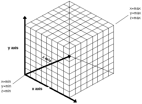
Figure 3-8 shows an example of a 3-D uniform lattice.
A 2-D image is an example of a uniform lattice; all the pixels in the image have the same size and aspect ratio. You can change the aspect ratio of a lattice by manipulating the bounding box coordinates.
For example, the lattice in Figure 3-7 has 5 by 9 nodes. The default mapping provides a 1:1 aspect ratio. Since the bounding box for this lattice is [0, 4] by
[0, 8], the lattice is mapped into a 5 by 9 grid to be displayed. However, if the bounding box coordinates were [-1, 1] by [-1, 1], the lattice would occupy a 2 by 2 space when mapped to the screen, with a pixel aspect ratio of 2:1. Uniform lattices can have this non-uniform aspect.
A perimeter lattice has a list of coordinate values sufficient to specify an irregularly spaced rectangular structure.
The data structure for a perimeter lattice is:
struct {
  long    sumCoord; /* Total number of nodes in all dims */
  float   *perimCoord; /* Ordered list of all coordinates */
} cx_coord_perimeter;
|
Figure 3-9 shows the data set for a 2-D perimeter lattice. The x and y perimeter vectors contain coordinate values that specify the layout of the lattice. It contains eight nodes in the x dimension and six nodes in the y dimension.

Coordinates for perimeter lattices are stored in row-major format in the C convention (see Figure 3-10).

Figure 3-11 shows an example of a 3-D perimeter lattice. The dims values are the same for each of the perimeter vectors, because there are eight nodes in each dimension.
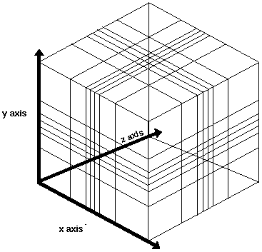
You can compute sumCoord by calling the API subroutine cxDimsSum. See the IRIS Explorer Reference Pages for details on the API subroutines. *perimCoord is an array of length sumCoord containing an ordered list of all the coordinates for each dimension.
Curvilinear lattices are used to define distorted shapes, such as flow patterns in fluid dynamics, or the surface variations of a sphere. The coordinate variable for a curvilinear lattice stores explicit coordinate values for each node in the lattice. There is no restriction on the range of values.
The data structure for a curvilinear lattice is:
struct {
      long  nCoordVar; /* Number of physical dimensions */
      float *values; /* Array containing node coordinates */
} cx_coord_curvilinear;
|
You can use cxDimsProd to compute the product of the dims vector.
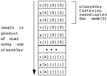
Coordinate values for curvilinear lattices are stored interlaced at the node level in the Fortran convention, with the I dimension varying the fastest. This is the reverse of the storage methods for uniform and perimeter coordinates.
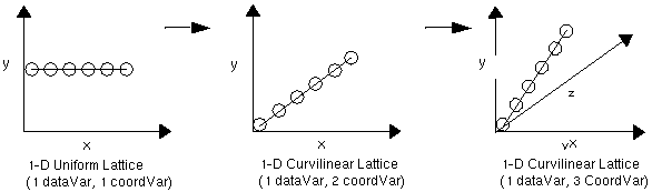
You can use a curvilinear lattice to depict the positions of data values in three dimensions. For example, the trajectory of a particle with time as the data variable can be described in a 1-D curvilinear lattice with the coordinates of each point in time as (x(t), y(t), z(t)), as shown in Figure 3-13.
Here, nDim is 1, dims is the number of time-steps, and nCoordVar is 3. The 1-D uniform lattice shows the same trajectory in a plane. As the trajectory moves out of the plane, each node must be defined by three coordinates, x, y and z. But there is still only one data value at each node.
In 1-D, perimeter and curvilinear lattices are structurally the same but their data values are stored differently in memory. Perimeter data values are stored in row-major format, and curvilinear data values are stored in column-major format (see Figure 3-4). The format matters when you set up an array data file for conversion into a lattice via the DataScribe™ (see “Preparing Your Data for Lattices” for more information) or to read into a module.
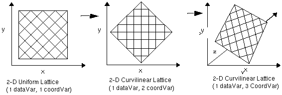
The shape of a non-uniform B-spline (NURBS) can be described in a 2-D curvilinear lattice. The two data variables are the dimensions of the spline field and the coordinates of each point are (x(t), y(t), z(t)). Here, nDim is 2, dims is the number of nodes, and nCoordVar is 3.
Figure 3-14 shows how a 2-D curvilinear lattice is aligned in three coordinate dimensions.
This is how you would set up cxLattice for a 2-D curvilinear lattice:
cxLattice
   nDim          1
   dims          # points
   cxData
     nDim, dims  (ditto)
     nDataVar    1 x
     primType    <...x
     values      Z[0],x Z[1], ...
    cxCoord
      nDim, dims (ditto)
      coordType  cx_coord_curvilinear
      nCoordVar  2
      values     [0], Y[0], X[1], Y[1], ...
|
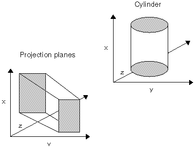
You can use 3-D curvilinear lattices to describe volumes. Figure 3-15 shows some examples of volumes.
When you build a module, you specify the range of lattice types the module can accept on its input port or produce on its output port. You can define in general terms the lattice constraints that encompass a large range of values for a given element, or you can be very specific. The range you choose will depend on the kind of data you want the module to handle.
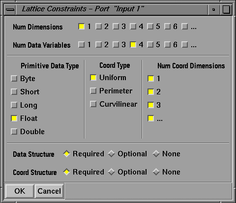
The Lattice Constraints window in Figure 3-16 shows the settings for a more narrowly defined lattice, such as a colormap (see “Lattice Examples”). The port will accept a 1-D lattice with four data variables. The primitive data type must be a float, and the lattice coordinate type must be uniform. The number of coordinate dimensions is not limited.
See “Defining Lattice Constraint Fields” for more information on using this window.
These examples show how to create some simple, commonly used lattices. They include code for a colormap and a 2-D image.
A colormap is a 1-D lattice with four variables per node (RGBA). Nodes are spaced uniformly. The data is usually in floating point format. The elements are:
| nDim | usually 1, although colormaps can be a function of more than one variable[4] | |
| dims | 256 | |
| nDataVar | 4 (red, green, blue, alpha) | |
| primType | float | |
| coordType | uniform |
See “Code Examples” for an example of a user function for a module that accepts a colormap.
An image is a 2-D lattice with one variable (greyscale), three variables (RGB), or four variables (RGBA) per node. The data is usually in byte format and the coordinate spacing between nodes is usually uniform. Explorer image-processing modules accept images of any size. The elements are:
| nDim | 2 | |
| dims | any | |
| nDataVar | 4 (red, green, blue, opacity) | |
| primType | byte | |
| coordType | usually uniform, although certain Landsat images and “fish-eye” photographic images may be distorted and therefore use curvilinear coordinates |
See “Code Examples” for examples of user functions for modules that work with both 2-D and 3-D lattices.
To prepare your data for input into an Explorer lattice data type, follow these points:
All information in the data portion of a lattice must be of only one of the primitive types. You cannot have a lattice that mixes primitive types, for example, having some bytes and some floats in one data file.
If you are coding in Fortran, remember to use zero-based indices instead of one-based indices.
If you have Fortran scalars, convert your primitive type into the equivalent Explorer primitive type (see “Defining Primitive Values”).
The coordinate data for uniform and perimeter lattices is stored differently from curvilinear lattices. Read the sections on these coordinate types to make sure you have your data values correctly arrayed.
For information on converting foreign data arrays into Explorer lattices, see Chapter 7, “Using the Parameter Data Type,”in the IRIS Explorer User's Guide.
The cxLattice data type, though defined in the Explorer typing language, can be considered as a C structure. Fortran users need to set pointers to the data type structures when they use them. The type declaration resides in the header file /usr/explorer/include/cx/cxLattice.h.
This is the cxLattice data type declaration:
#include <cx/Typedefs.h>

typedef enum {
    cx_coord_uniform,
    cx_coord_perimeter,
    cx_coord_curvilinear
} cxCoordType;

typedef struct cxCoord {
    long             nDim;           /* arg 0 */
    long             *dims;          /* arg 1 */
    cxCoordType      coordType;
    union {
       struct {
          float            *bBox;
        } cx_coord_uniform;
        struct {
           long              sumCoord;
           float            *perimCoord;
        } cx_coord_perimeter;
        struct {
           long              nCoordVar;
           float            *values;
        } cx_coord_curvilinear;
    } c;
} cxCoord;

typedef struct cxData {
    long              nDim;           /* arg 0 */
    long             *dims;           /* arg 1 */
    long              nDataVar;
    cxPrimType        primType;
    union {
        struct {
            unsigned char    *values;
        } cx_prim_byte;
        struct {
            short            *values;
        } cx_prim_short;
        struct {
            long             *values;
        } cx_prim_long;
        struct {
            float            *values;
        } cx_prim_float;
        struct {
            double           *values;
        } cx_prim_double;
    } d;
} cxData;

typedef struct cxLattice {
    long              nDim;
    long             *dims;
    cxData           *data;
    cxCoord          *coord;
} cxLattice;
|
The Fortran type enumerations reside in the file /usr/explorer/include/cx/cxLattice.inc.
The three coordinate mappings are specified as follows:
integer cx_coord_uniform integer cx_coord_perimeter integer cx_coord_curvilinear parameter (cx_coord_uniform = 0 ) parameter (cx_coord_perimeter = 1 ) parameter (cx_coord_curvilinear = 2 ) |
| Note: All Fortran data type access routines use zero-based indexing, as in the C language (except where otherwise stated). |
You can use the API (Application Programming Interface) routines to manipulate data types in Explorer. The lattice subroutines are listed below and described in detail in the IRIS Explorer Reference Pages. They let you:
create a lattice with both data and coordinates, either one, or neither
calculate the size of the data set
set lattice values
copy a source lattice (or parts thereof) and allocate it to the destination
extract specific values or descriptive information from the lattice
Some routines check the validity of the data on the inputs before the module is fired. Table 3-2 lists the subroutines and briefly describes the purpose of each one.
Table 3-2. Lattice Subroutines
Subroutine | Purpose |
|---|---|
cxLatNew | Creates a lattice with data and coordinates |
cxLatDataNew | Creates a lattice with data and no coordinates |
cxLatCoordNew | Creates a lattice with coordinates and no data |
cxLatRootNew | Creates a lattice with no data and no coordinates |
cxDataNew | Creates new data structure |
cxCoordNew | Creates new coordinate data structure |
cxCoordDefaultNew | Creates default index coordinates |
cxDataPrimSize | Returns the size of the primitive data type |
cxDataPrimType | Returns the primitive data type |
cxCoordType | Returns the lattice coordinate type |
cxDimsProd | Returns the total number of data points in a lattice |
cxDimsSum | Computes the sum of a dimensions vector (for perimeter lattices only) |
cxLatPtrSet | Sets lattice data and coordinate pointers |
cxLatPtrGet | Gets pointers to lattice data and coordinates |
cxLatDup | Duplicates a lattice with data or coordinates |
cxLatRootDup | Duplicates a lattice without data or coordinates |
cxDataDup | Duplicates data values |
cxCoordDup | Duplicates coordinates |
cxLatDescGet | Gets descriptive information about a lattice |
cxDataValsGet | Returns pointer to data values |
cxDataValsSet | Sets pointer to data values |
cxCoordValsGet | Returns pointer to coordinate value |
cxCoordValsSet | Sets pointer to coordinate values |
cxCoordNVarGet | Gets number of coordinate variables |
cxCoordNVarSet | Sets number of coordinate values |
This section presents three examples of source code using the lattice data structure. Each one is written in C and in Fortran. The source code files and modules for all the examples reside in /usr/explorer/src/MWGcode.
This example shows how to create a a simple colormap module. The code resides in /usr/explorer/src/Lattice/C/ColorMap.c and in /usr/explorer/src/Lattice/Fortran/ColorMap.f.
#include <stdio.h>

#include <cx/DataAccess.h>
#include <cx/cxLattice.h>
#include <cx/cxLattice.api.h>

/*
 This user function takes a colormap input (1-D lattice with 4 floats
 per sample) and inverts the red, green, and blue components of each
 lookup value.
*/
void cchange(
cxLattice *cin, 							/* input colormap lattice */
cxLattice **cout) 							/* output colormap lattice */
{
   int    i;     /*loop variable */
   int      n;     /* number of colormap entries */
   float    *a,*b; /* pointers to colormap data */
   cxErrorCode err;

   /* create the new lattice */
  *cout = cxLatDataNew(
     1, 					/* number of dimensions */
     cxLatticeDimensionsArrayGet(cin,&err),
     4,    					/* number of data values */
     cx_prim_float); 					/* data type */

     /* use the same coordinate space as the input lattice */
     cxLatPtrSet(*cout,NULL,NULL,
     cxLatticeCoordStructureGet(cin,&err),NULL);

     /* get the number of samples */
     n = (int)*cxLatticeDimensionsArrayGet(cin,&err);

     /* get the data pointers */
     cxLatPtrGet(cin,NULL,(void **)&a,NULL,NULL);
        cxLatPtrGet(*cout,NULL,(void **)&b,NULL,NULL);

        /* invert the colors of the colormap entries */
        for ( i = 0; i < n; i++ )

                b[0] = 1.0 - a[0];    /* red */
                b[1] = 1.0 - a[1];    /* green */
                b[2] = 1.0 - a[2];    /* blue */
                b[3] = a[3];          /* alpha */

                a += 4; b += 4;
 		}
}
|
c
c       This user function takes a colormap input (1-D lattice with 4 real
c       values per sample) and inverts the red, green, and blue components
c     of each lookup value.
c
      subroutine fchange(cin,cout)

      integer cin       ! input colormap lattice
      integer cout      ! output colormap lattice

#include <cx/Typedefs.inc>
#include <cx/DataAccess.inc>

      integer i         ! loop variable
      integer n(1)      ! number of colormap entries
      integer nn        ! need this variable because of a compiler bug
      integer coord     ! coordinate pointer
      real    a(1),b(1) ! colormap data
      integer err

      pointer (pa,a)
      pointer (pb,b)
      pointer (pn,n)

      ! get the number of samples
      call cxLatDescGet(cin,tmp,pn,tmp,tmp,tmp,tmp,tmp,tmp)
      nn = n(1)

      ! create the new lattice
      cout = cxLatDataNew(
     +  1,
     +  n,
     +  4,
     +  cx_prim_float)

      ! use the same coordinate space as the input lattice
      call cxLatPtrGet(cin,tmp,tmp,coord,tmp)
      call cxLatPtrSet(cout,0,0,coord,0)

      ! get the data pointers
      	 ! (Note that we *could* have just had the data pointers passed into
      	 !  the user function as arguments, which is probably easier.)
      call cxLatPtrGet(cin,tmp,pa,tmp,tmp)
      call cxLatPtrGet(cout,tmp,pb,tmp,tmp)

      ! invert the red, green, and blue lookup values
      do i = 1,nn
          b(4*i - 3) = 1.0 - a(4*i - 3)
          b(4*i - 2) = 1.0 - a(4*i - 2)
          b(4*i - 1) = 1.0 - a(4*i - 1)
          b(4*i) = a(4*i)
      end do

      return
      end
|
This example shows how to work with a 2-D image. The code resides in /usr/explorer/src/Lattice/C/Image2D.c and in /usr/explorer/src/Lattice/Fortran/Image2D.f.
#include <stdio.h>

#include <cx/DataAccess.h>
#include <cx/cxLattice.h>
#include <cx/cxLattice.api.h>

/*
 This user function takes an input 2-D image and negates all the
 elements of the data array. It works for any primitive data
 type.  */
void cimage(cxLattice *in,cxLattice **out)
{
      int  i,j,k;                /* loop variables */
      void *a,*b;                /* data pointers */
      cxErrorCode err;

  /*create the new lattice */
  *out = cxLatDataNew(
     2,                    /* number of dimensions */
     in->dims,             /* dimensions array */
     in->data->nDataVar,   /* number of data variables */
     in->data->primType);  /* data type */

/ * use the same coordinate space as the input lattice */
 exLatPtrSet(*out,NULL,NULL,cxLatticeCoordStructureGet(in,&err),NULL);

/* extract the data pointers */
  cxLatPtrGet(in,NULL,&a,NULL,NULL);
 		 cxLatPtrGet(*out,NULL,&b,NULL,NULL);

 /*loop over the data elements */
   for ( i = 0; i < in->dims[1]; i++ )
      for ( j = 0; j < in->dims[0]; j++ )
         for ( k = 0; k < in->data->nDataVar; k++ )
         {
           /* switch on the data type */
          /*
          /*This should be outside the loops for efficiency.     It is shown inside here for greater clarity./

          switch ( in->data->primType )
 {
  #define CASE(CXTYPE,TYPE) \
    case CXTYPE: \
       /* This is where the actual computation takesplace*/\
       *TYPE *)b = -*(TYPE *)a; \
       a = (TYPE *)a + 1; b = (TYPE *)b + 1; \
       break;
           CASE(cx_prim_byte,unsigned char)
           CASE(cx_prim_short,short)
           CASE(cx_prim_long,long)
        CASE(cx_prim_float,float)
        CASE(cx_prim_double,double)
        default:
               break;
#undef CASE

    }
 }
|
c
c       This user function takes an image input (2-D lattice of any data
c     type) and takes the negative of every data element.
c
      subroutine fimage(in,out)

      integer in        ! input image
      integer out       ! output image

#include <cx/Typedefs.inc>
#include <cx/DataAccess.inc>

      integer i,j,k     ! loop variables
      integer n,m,p     ! utility variables

      integer dims(1)   ! dimensions vector for lattice
      integer nDataVar  ! number of data variables
      integer primType  ! data type
      integer coord     ! coordinate structure
      pointer (pdims,dims)
      integer*1 b0(1),b1(1)    ! arrays for each primitive type
      integer*2 s0(1),s1(1)
      integer*4 l0(1),l1(1)
      real f0(1),f1(1)
      double precision d0(1),d1(1)
      pointer (pb0,b0)
      pointer (pb1,b1)
      pointer (ps0,s0),(ps1,s1)
      pointer (pl0,l0),(pl1,l1)
      pointer (pf0,f0),(pf1,f1)
      pointer (pd0,d0),(pd1,d1)

      ! extract information from the input lattice
        call cxLatDescGet(in,tmp,pdims,tmp,nDataVar,primType,tmp,tmp,tmp)

      ! compiler bug requires this hack
      n = dims(2)
      m = dims(1)

      ! create the new lattice
      out = cxLatDataNew(2,dims,nDataVar,primType)

      ! use the same coordinate space as the input lattice
      call cxLatPtrGet(in,tmp,tmp,coord,tmp)
      call cxLatPtrSet(out,0,0,coord,0)

      ! extract data pointers based on primitive type
      if ( primType .eq. cx_prim_byte ) then
          call cxLatPtrGet(in,tmp,pb0,tmp,tmp)
          call cxLatPtrGet(out,tmp,pb1,tmp,tmp)
      else if ( primType .eq. cx_prim_short ) then
          call cxLatPtrGet(in,tmp,ps0,tmp,tmp)
          call cxLatPtrGet(out,tmp,ps1,tmp,tmp)
      else if ( primType .eq. cx_prim_long ) then
          call cxLatPtrGet(in,tmp,pl0,tmp,tmp)
          call cxLatPtrGet(out,tmp,pl1,tmp,tmp)
      else if ( primType .eq. cx_prim_float ) then
          call cxLatPtrGet(in,tmp,pf0,tmp,tmp)
          call cxLatPtrGet(out,tmp,pf1,tmp,tmp)
      else if ( primType .eq. cx_prim_double ) then
          call cxLatPtrGet(in,tmp,pd0,tmp,tmp)
          call cxLatPtrGet(out,tmp,pd1,tmp,tmp)
      endif
! loop over all the data items
      p = 1
      do i = 1,n
          do j = 1,m
              do k = 1,nDataVar
                  ! do the computation
                  !   The data type switching should be outside the loop
                  !   for efficiency.  It is shown inside here for greater
                  !   clarity.
                  if ( primType .eq. cx_prim_byte ) then
                      b1(p) = -b0(p)
                  else if ( primType .eq. cx_prim_short ) then
                      s1(p) = -s0(p)
                  else if ( primType .eq. cx_prim_long ) then
                      l1(p) = -l0(p)
                  else if ( primType .eq. cx_prim_float ) then
                      f1(p) = -f0(p)
                  else if ( primType .eq. cx_prim_double ) then
                      d1(p) = -d0(p)
                  endif

                  p = p + 1     ! increment the data item
              end do
          end do
      end do

      return
      end
|
This example illustrates how to create a curvilinear lattice and rotate the coordinates. The code resides in /usr/explorer/src/Lattice/C/Curvi3D.c and in /usr/explorer/src/Lattice/Fortran/ICurvi3D.f.
#include <stdio.h>
#include <math.h>
#include <cx/DataAccess.h>
#include <cx/DataExtract.h>
#include <cx/cxLattice.h>
#include <cx/cxLattice.api.h>


void cwind(float rot,cxLattice *in,cxLattice **out)
{
       int     i,j,k;          /* loop variables */
          int       index[3];           /* index vector for coordinate lookup */
          float     *c;               /* pointer to output lattice coordinates */
        float   coord[3];       /* input coordinate vector */
        float   cosa,sina;      /* utility variables */

        /* create the new lattice */
        *out = cxLatCoordNew(
        3,                      /* number of dimensions */
        in->dims,               /* dimensions array */
        3,                      /* coordinate dimensions */
        cx_coord_curvilinear);  /* type of coordinates */

        /* use the same data from the input lattice */
        cxLatPtrSet(*out,in->data,NULL,NULL,NULL);

        /* get the coordinate data pointer */
        cxLatPtrGet(*out,NULL,NULL,NULL,(void **)&c);

        /* loop over the elements */
        for ( i = 0; i < in->dims[2]; i++ )
        {
             index[2] = i;   /* set z index */

             for ( j = 0; j < in->dims[1]; j++ )
             {
                  index[1] = j;   /* set y index */

                  for ( k = 0; k < in->dims[0]; k++ )
                  {
                       index[0] = k; /* set x index */

                       /* get the original coordinates */
                       cxLatCoordExtract(in,index,coord);
                             /* wind the coordinates around the z-axis */
                       cosa = cos(rot*coord[2]);
                       sina = sin(rot*coord[2]);

                       c[0] = coord[0]*cosa + coord[1]*sina;
                       c[1] = coord[0]*sina - coord[1]*cosa;
                       c[2] = coord[2];

                       /* increment pointer */
                       c += 3;
                     }
             }
      }
}
|
      subroutine fwind(rot,in,out)

      real      rot
      integer   in
      integer   out

#include <cx/Typedefs.inc>
#include <cx/DataAccess.inc>
#include <cx/cxLattice.inc>

      integer i,j,k     ! loop variables
      integer nx,ny,nz
      integer m
      integer dims(1)   ! dimensions array
       integer index(3)  ! index array for extracting coordinates
      integer d         ! data structure
      real    coord(3)  ! input coordinate vector
      real    c(1)      ! output coordinate array
      real    cosa,sina

      pointer (pdims,dims)
      pointer (pc,c)

      ! get the dimensions vector
      call cxLatDescGet(in,tmp,pdims,tmp,tmp,tmp,tmp,tmp,tmp)
      nx = dims(1)
      ny = dims(2)
      nz = dims(3)

      ! create the new lattice
      out = cxLatCoordNew(3,dims,3,cx_coord_curvilinear)

      ! use the same data as the input lattice
      call cxLatPtrGet(in,d,tmp,tmp,tmp)
      call cxLatPtrSet(out,d,0,0,0)

      ! get the output data pointer
      call cxLatPtrGet(out,tmp,tmp,tmp,pc)

      ! loop over the coordinates
      m = 1
      do i = 1,nz
          index(3) = i - 1      ! set z index (0 based for api routine)

          do j = 1,ny
              index(2) = j - 1          ! set y index

              do k = 1,nx
                  index(1) = k - 1              ! set x index

                  ! get the original coordinates
                  call cxLatCoordExtract(in,index,coord)

                  ! wind the coordinates around the z-axis */
                  cosa = cos(rot*coord(3))
                  sina = sin(rot*coord(3))

                  c(m) = coord(1)*cosa + coord(2)*sina
                  c(m + 1) = coord(1)*sina - coord(2)*cosa
                  c(m + 2) = coord(3)

                  ! increment index
                  m = m + 3
              end do
          end do
      end do

      return
      end
|
[4] If you use a 2-D colormap, you must create your own modules to process it. Explorer currently offers tools for 1-D colormaps only.