This chapter describes how you can use compounds (or conversely, decomposition) to scale the performance of your graphics system. Decomposition allows you to use multiple pipes to render frames that would normally be rendered by a single pipe.
This chapter has the following sections:
To achieve greater application performance, MPK allows you to decompose a global rendering task into smaller tasks and to assign the smaller tasks to individual pipes. The task division requires a decomposition scheme. In general, a decomposition scheme sends a scene to render to each pipe, gets back rendered images from each pipe for further composition, and then renders the final image. An exception is cull decomposition, where the cull operation is parallelized with the draw operation.
Figure 4-1 illustrates the role of source and destination channels in scalable rendering.
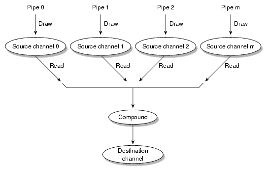
To build a compound, you must create a c ompound data structure. Chapter 6, “Configuration File Format” describes the syntax of compound data structures for your configuration file. This section describes how you build them logically.
Generally, to create a compound, you need to do the following:
Choose a decomposition scheme, which divides the global rendering task into smaller tasks.
Distribute the rendering of the smaller tasks to the source pipes for parallel processing.
Designate a destination channel for the reassembly of the final, coherent image.
The destination channel is usually one of the source channels. To achieve optimal performances, you would usually have one channel per pipe.
This chapter focuses on the three tasks just cited. Optionally, you can also do the following:
The section “Stereo-Selective Compounds” describes how you control whether your compound is used depending on the stereo mode of the application. For more information on the first two optional tasks, see the descriptions of the mode and format fields in section Chapter 6, “Configuration File Format”. Chapter 5, “Using Scalable Graphics Hardware” describes the integration of scalable graphics with MPK. “Automatic Load Balancing for Compounds” describes how MPK balances the rendering for certain compound modes.
MPK provides several decomposition schemes and the following subsections describe these schemes:
Each decomposition mode improves performance or graphics quality, but the performance gain depends on the application type and the nature of the performance bottleneck. Four factors are important in choosing the decomposition scheme judiciously:
In frame decomposition, a frame or view is divided into regions, which are, in turn, assigned to individual source pipes for rendering. Based on the following perspectives, there are several approaches to dividing the frame into regions:
Screen topology (screen decomposition)
Scene graph primitives (database decomposition)
Eye view (eye decomposition)
Each approach yields a different flavor of frame decomposition.
In screen decomposition (also referred to as 2D decomposition), each pipe renders a part of the screen area. Assembling side-to-side each image part constitutes the final rendering. This type of decomposition is used when the intrinsic pixel fill or geometry capacity of each pipe slows down the application. The scalability depends on the balancing of the workloads. The model to display needs to be uniformly distributed across the screen to accommodate a good balancing and, thus, scalability. The graphics I/O is relatively low, because the traveling source images are small.
Figure 4-2 illustrates screen decomposition.
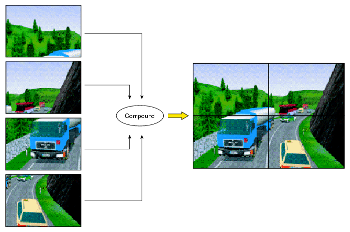
Example 4-1 shows the configuration file specifications for the screen decomposition illustrated in Figure 4-2.
Example 4-1. 2D Compound in a Configuration File
compound {
    mode [2D]
    channel "destination"

# The top left of "destination" image will be
# rendered on "source0"...
    region {
        viewport [ 0., .5, .5, .5 ]
        channel "source0"
    }
# The top right of "destination" image will be
# rendered on "source1"...
    region {
        viewport [ .5, .5, .5, .5]
        channel "source1"
    }
# The bottom left of "destination" image will be
# rendered on "source2"...
    region {
        viewport [ 0., 0., .5, .5 ]
        channel "source2"
    }
# ... while "destination" itself takes care of
# the bottom right
    region {
        viewport [ .5, 0., .5, .5 ]
        channel "destination"
    }
}
|
A 2D compound has no frame latency, unless the mode flag ASYNC has been set, in which case the latency is one frame but you get better overall performance.
In database (DB) decomposition, the scene is rendered in parallel by dividing it among the different graphics pipes. Each pipe renders its share of the scene to generate partial images. These images are then composited by MPK to generate the final image in the destination channel. During composition, the application can use depth testing and/or alpha blending to achieve the desired effect. Database decomposition allows you to scale both the geometry and the pixel fill performance of the system. For some applications, such as volume rendering, it also scales the texture memory capacity of the system by the number of pipes.
Figure 4-3 demonstrates the use of database decomposition in volume rendering. The volume data is divided equally among the four pipes and the partial images are composited on the destination channel. In this case, the destination channel (top left portion of the figure) is also contributing to the rendering as a source channel.
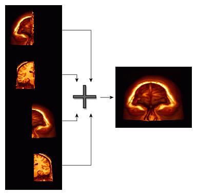
Example 4-2 shows the configuration file specifications for the database decomposition illustrated in Figure 4-3.
Example 4-2. DB Compound in a Configuration File
compound {
    mode    [ DB ]
    format  [ COLOR DEPTH ]
    channel “channel”

    region {
        range       [ 0., .25 ]
        channel     “buffer0”
    }

    region {
        range       [ .25, .5 ]
        channel     “buffer1”
    }

    region {
        range       [ .5, .75 ]
        channel     “buffer3”
    }

    region {
        range       [ .75, 1. ]
        channel     “channel”
    }
}
|
The application must support the DB compound.
Eye decomposition is well-suited for stereo or multiple-view rendering. Each pipe renders a particular view (left, right, mono). The final rendering depends on the type of display. As illustrated in Figure 4-4, if stereo is active, then each pipe view fills in the right or left buffer of the final rendering. This provides good load balancing and scalability, especially for stereo-view rendering, because the scene content remains similar during run time.
An EYE compound has no frame latency, unless the mode qualifier ASYNC has been specified and pixel transfer needs to occur, in which case the latency is 1.
The number of regions of an eye compound is not limited. If more than one region correspond to the same eye view, MPK uses the first specified region (for this eye) as source for the pixel transfer, if needed.
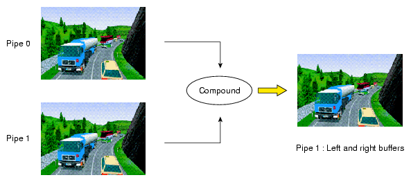
Example 4-3 shows the configuration file specifications for the eye decomposition illustrated in Figure 4-4.
Example 4-3. Eye Compound in a Configuration File
compound {
        mode    [ EYE STEREO ]
        channel “channel”

        region {
            eye         LEFT
            channel     “buffer”
        }

        region {
            eye         RIGHT
            channel     “channel”
        }
}
|
Head-Mounted-Device (HMD) decomposition is very similar to that of eye decomposition, except that the head position actually specifies a new origin for the physical layout of the channels.
Example 4-4 shows a configuration file specification for an HMD decomposition:
Example 4-4. HMD Compound in a Configuration File
compound {
    mode [HMD]
    channel “destination”

    region {
        eye     left
        channel “source::left”
    }

    region {
        eye     right
        channel “source::right”
    }
}
|
If a destination channel is specified, then the frustum is inherited from the destination channel's wall or projection frustum specification; otherwise, the source channel's frustum specification will be used.
In contrast to frame decomposition, where the focus of load balancing is on dividing the frame into regions, temporal decomposition balances the workload by scheduling the work on each pipe in sync with that of the other pipes to produce a steady stream of rendered frames. The time scheduling rather than the frame division is the focus. There are two types of temporal decomposition: frame multiplexing and data streaming. The work done by each pipe largely distinguishes the two.
Frame multiplexing (also referred to as DPLEX decomposition) distributes entire frames to the source pipes over time for parallel processing. The first pipe begins rendering frame 1; a specified fraction of a frame later the second pipe begins rendering frame 2; another fraction of a frame later the third pipe begins rendering frame 3; and so on for all of the pipes.
Figure 4-5 illustrates frame multiplexing on a four-pipe system.
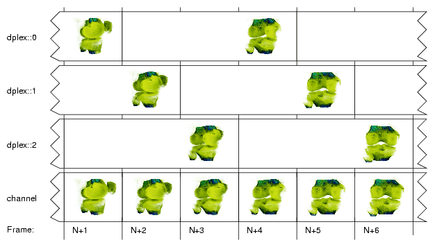
Frame multiplexing globally scales geometry and pixel fill performance, as the workload balance between pipes is intrinsically maintained. This scheme has an increased transport delay inherent to frame synchronization required across the pipes. It produces a latency of (pipes – 1) frames—that is, there will be a (pipes – 1) frames delay between a user input and the corresponding output frame.
Frame multiplexing can also be accelerated in hardware using the SGI Scalable Graphics Compositor, which connects pipes together with a bus, thereby avoiding the image readbacks from the contributing pipes. The pipes are daisy-chained to achieve reduced latency. For more details, see Chapter 5, “Using Scalable Graphics Hardware”.
Example 4-5 shows the configuration file specifications for the frame multiplexing decomposition illustrated in Figure 4-5. The application must support the DPLEX compound.
Example 4-5. DPLEX Compound in a Configuration File
compound {
    mode    [ DPLEX ]
    channel “channel”

    region {
        channel “dplex::0”
    }

    region {
        channel “dplex::1”
    }

    region {
        channel “dplex::2”
    }
}
|
Data streaming (also referred to as 3D decomposition) is similar to database decomposition in that it allows the application to divide the scene among multiple pipes and then composite the partial results to give the final rendering. But, in this case, the composition is done using a series of successive compounds for each frame, as shown in Figure 4-6. For frame N+1, channel stream::1 draws the first quarter of the database, which is copied to channel stream::2 at the beginning of the next frame. During frame N+2, channel stream::2 draws the second quarter of the database on top while channel stream::1 starts a new frame. At frame N+4, the destination channel channel finishes drawing the last quarter and displays the frame started three time steps ago.
Like DPLEX decomposition, this scheme also has a latency of (pipes – 1) frames—that is, there will be a (pipes – 1) frames delay between a user input and the corresponding output frame. As shown in Figure 4-6, this latency is due to successive compounds at each frame. You must wait for (pipes – 1) frame computations before the final rendering is displayed. Each compound needs to read only one source image. Consequently, this keeps graphics I/O consumption low while performance scaling is achieved by pipelining the rendering in parallel across the pipes.

As shown in Example 4-6, the configuration file specification for a data streaming decomposition is similar to that for database decomposition.
Example 4-6. Data Streaming Compound (3D) in a Configuration File
compound {
    mode    [ 3D ]
    format  [ COLOR DEPTH ]
    channel “channel”

    region {
        range      [ .0 .25 ]
        channel    “stream::1”
    }

    region {
        range      [ .25 .5 ]
        channel    “stream::2”
    }

    region {
        range      [ .5 .75 ]
        channel    “stream::3”
    }

    region {
        range      [ .75 1. ]
        channel    “channel”
    }
}
|
The application must support the 3D compound.
In pixel-based decomposition, a frame is rendered using a multipass approach where single passes are assigned to individual source pipes for rendering. Assembling each frame using accumulation techniques constitutes the final rendering. Accumulation of the frames can be achieved using one of the following techniques:
In order to use OpenGL accumulation, you must use an appropriate visual; otherwise, MPK uses blending.
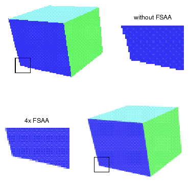
MPK has implemented one scheme of pixel-based decomposition, a full-scene antialiasing (FSAA) compound. Each pipe renders the full scene from a slightly different viewpoint. The number of rendering passes of a FSAA compound is defined by its number of sources. Furthermore, every channel can thereby be used multiple times. This type of decomposition is used when the the resulting output quality has highest priority. The scalability and final rendering quality depends on the number of available pipes.
Example 4-7 shows an FSAA compound using the SGI Scalable Graphics Compositor:
Example 4-7. Four-Pipe 4x FSAA Compound Using the SGI Graphics Compositor
compound {
    mode    [ FSAA HW NOCOPY ]
    channel “channel-0”

    # The number of sources defines the FSAA mode
    region {
        channel “channel-0”
    }
    region {
        channel “channel-1”
    }
    region {
        channel “channel-2”
    }
    region {
        channel “channel-3”
    }
}
|
Figure 4-7 illustrates the advantage of using a 4x FSAA solution.
Example 4-8 shows how to use the same channel multiple times as a source channel to support multipass rendering in MPK on machines with only a few pipes.
Example 4-8. Multiple Use of a Single Channel in FSAA Decomposition
compound {
    mode    [ FSAA ]
    channel “channel”

    # The number of sources defines the FSAA mode
    region {
        channel “channel”
    }
    region {
        channel “channel”
    }
    region {
        channel “channel”
    }
    region {
        channel “channel”
    }
}
|
Cull decomposition is different from the other decomposition modes in that it does not decompose the rendering of a frame. Instead, it decomposes (parallels) the cull and draw operations. Naturally, the use of this feature in the configuration file requires the application also to support the cull decomposition mode.
In cull decomposition, a region specifies the operation to be executed by this region. Example 4-9 shows a cull decomposition for a single channel.
Example 4-9. A Simple Cull Decomposition
config
{
    name    “1-window”

    pipe
    {
        window
        {
            name        “MPK: simple”
            viewport    [ 0.25, 0.25, 0.5, 0.5 ]

            channel
            {
                name        “channel”

                wall
                {
                    bottom_left     [ -.5, -.4, -1 ]
                    bottom_right    [  .5, -.4, -1 ]
                    top_left        [ -.5,  .4, -1 ]
                }
            }
        }
        window
        {
             attributes { hints { drawable none } }
             channel    { name    “cull” }
        }
    }

    compound
    {
         mode [ CULL ]
         channel “channel”

         region { cull channel “cull”    }
         region { draw channel “channel” }
    }
}
|
In this example, the channel cull executes the culling concurrently with the draw operation of channel channel. It is defined on a window that has no drawable, because it is not used for any draw operation. You can add the ASYNC flag to force the cull region to process data for the frame N, and the draw region to draw frame N–1. This introduces an additional frame of latency, but potentially increases performance.
The region operation can be the value cull, draw, or cull-draw. The default operation is cull-draw; that is, all source channels first execute the cull operation and then the draw operation.
If multiple regions of a cull compound execute the same operation (cull or draw) for the destination channel, they process the data in parallel and, therefore, may speed up the operation if enough resources are available. As a feature of the MPK implementation, the distribution of the cull and draw tasks is automatically load-balanced. For recomposition, MPK uses by default the same algorithm that is used for DB compounds.
 | Note: Since culling is application-specific, you must determine (perhaps, from your application vendor) what MPK features and configurations are supported by your application. |
It is possible to further decompose the regions of a cull compound, as described in the following section, “Multilevel Decomposition”.
MPK allows you to combine the various decomposition schemes to fix performance bottlenecks that differ in nature. For example, a combined solution can use a database and temporal decomposition scheme for optimizing performance (but it will have a limiting transport delay) or can use an eye and database decomposition scheme for stereo volume rendering.
Figure 4-8 shows a four-pipe solution using an eye and database decomposition scheme.
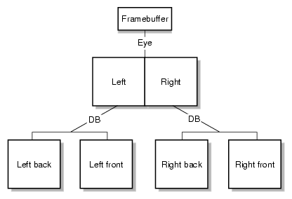
Example 4-10 shows the configuration file specifications for the multilevel decomposition illustrated in Figure 4-8.
Example 4-10. Multilevel Compound in a Configuration File
compound {
    mode    [ EYE ]
    channel “right-front”

    region {
        eye    LEFT
        compound {
            mode    [ DB ]
            channel “left-front”

            region {
                range   [ 0., .5 ]
                channel “left-back”
            }

            region {
                range   [ .5, 1. ]
                channel “left-front”
            }
        }
    }

    region {
        eye    RIGHT
        compound {
            mode    [ DB ]
            channel “right-front”

            region {
                range   [ 0., .5 ]
                channel “right-back”
            }

            region {
                range   [ .5, 1. ]
                channel “right-front”
            }
        }
    }
}
|
In many instances, it will be desirable to control which compounds will be used by the application based on whether the application is running in stereo mode. MPK provides a mode parameter for this purpose. For instance, if the application is to run in stereo mode, you may want to use eye decomposition and when in mono mode, to use another type of decomposition. Example 4-11 illustrates this conditional use of compounds.
Example 4-11. Stereo-Selective Compounds
compound {
    mode    [ EYE STEREO ]
    channel “channel”

    region {
        eye         LEFT
        channel     “buffer”
    }
    region {
        eye         RIGHT
        channel     “channel”
    }
}

compound {
    mode    [ 2D MONO ]
    channel “channel”

    region {
        viewport    [ 0., 0., 1., .5 ]
        channel     “buffer”
    }

    region {
        viewport    [ 0., .5, 1., .5 ]
        channel     “channel”
    }
}
|
The MONO and STEREO flags allow you to specify different channel decompositions depending on the current configuration mode. This is especially useful for eye decomposition. In this example, when the destination channel is in stereo mode, MPK uses the eye decomposition. When the destination channel is in mono mode, MPK uses the 2D decomposition.
Achieving an ideal decomposition among the children of a compound can be difficult, since the workload per child often changes on a per-frame basis. To address this problem, MPK provides automatic load balancing for 2D, DB, and 3D compounds.
This section describes the following topics:
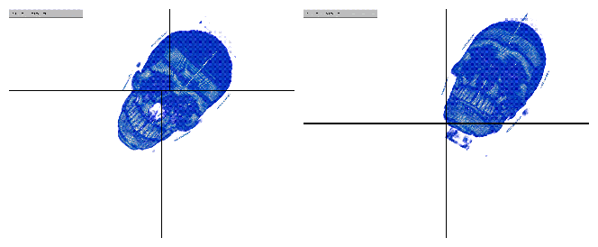
Figure 4-9 contrasts dynamic and static load balancing for a 2D compound using volview. Volume rendering is bound by fill rate; therefore, the load balancing can adjust the compound's region so that each pipe has approximately the same amount of volume to rasterize. When using static tiling, one pipe may have to render the whole volume as it is moved around. Since the slowest child dictates overall performance, the frame rate is better, in this case, when using load balancing.
Using the rendering times for each child, MPK computes a new viewport or range each frame. This approach needs the following conditions to work properly:
| Condition | Description | |
| Low latency | A new workload can only be computed after all children have drawn. Therefore, the higher the latency, the higher the difference will be between the frame which is used to compute the new balance and the frame for which the balance is computed. Logically, high latency is counterproductive in achieving proper load balancing. | |
| Frame consistency | Since the new viewport or range is computed based on the last finished frame but applied to the next frame, the two frames should be similar. This is true for most applications. | |
| Scalable compound mode | The chosen decomposition mode has to solve the application's bottleneck. For example, load balancing a 2D compound for a geometry-limited application will fail, unless this application uses view-frustum culling. | |
| Imbalance in decomposition | If the decomposition is already well-balanced—for example, for a DB compound—the static compound may provide a better frame rate. |
In the configuration file, you can use the ADAPTIVE mode flag for a compound to enable load balancing. This mode flag can be used for 2D, DB, and 3D compounds. 2D compounds will use tiles, while DB and 3D compounds will adapt the z-axis range to decompose the rendering. The next section describes how you use a split-axis method to determine tiling schemes and z-axis splits.
| Note: If you do not provide a tiling scheme (or z-axis split) for ADAPTIVE mode, MPK creates one. |
As the name implies, a split-axis method uses splits on the Cartesian coordinate axes to determine tiling schemes (or z-axis range splits). As noted in the preceding section, the tiling schemes are specific to 2D compounds and z-axis splits, to DB and 3D compounds.
You specify a split in the configuration file by using the split field of the compound data structure. Chapter 6, “Configuration File Format” describes the formal syntax for the split field. This section provides several examples of how to use the field. Example 4-12 shows a tiling scheme for a 2D compound with four regions (source channels) defined.
Note the following syntax items and other restrictions:
The split value is a string.
MPK uses the following operators in the string to denote the axis-specific splits:
| Splits the x axis.
– Splits the y axis.
/ Splits the z axis.
The operators | and – can be used only with 2D compounds and /, only with DB and 3D compounds.
Integers represent the regions in the compound data structure in the order of declaration. All regions declared in the compound must appear in the split string.
A set of brackets must enclose a split, which can be nested in another split (as shown in Example 4-12).
Figure 4-10 illustrates the tiling scheme specified in Example 4-12.
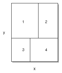
Example 4-13 , like Example 4-12, shows a tiling scheme for a 2D compound with four regions, but this time the primary split is on the x axis.
Figure 4-11 illustrates the tiling scheme specified in Example 4-13.
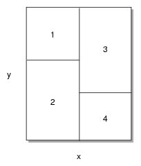
If you do not specify a split, MPK will automatically create one.
There are no hard and fast rules for choosing the correct decomposition scheme, but the following are some general guidelines to aid you in selecting a reasonable scheme for your environment:
| Mode | Recommended Use | |||
| 2D | Use this scheme if your application is fill-limited.You can also scale geometry performance and texture memory if your application is using view-frustum culling techniques. | |||
| 3D | Use this scheme where you would normally use the DB scheme but where you experience scalability problems caused by a graphics I/O bottleneck on the destination pipe. For 3D decomposition, the graphics I/O per pipe is constant when changing the number of contributing pipes. Unlike the DB scheme, however, adding pipes to a 3D compound increases latency. | |||
| DB | Use this scheme when your application's frame rendering can be sequenced into equally consuming phases. This requires the application to divide your scene into multiple components and then to composite them correctly. Scalability here can be either on fill, geometry, or graphics resources (texture) depending on the application. | |||
| FSAA | Use this scheme if graphics quality is a primary concern. | |||
| EYE | Use this scheme for stereo viewing. | |||
| DPLEX | Use this scheme for general load balancing where the application maintains a reasonably steady frame rate.
|
These are very high-level guidelines that may very well overlap. As noted in the section “Multilevel Decomposition”, you can combine the various decomposition modes to fix different performance bottlenecks.