This chapter discusses the features and capabilities of the Column Importance mining tool, and the relationship between column importance and the importance ranking in the other data mining tools. Because of the differences in representation for classification models, different attributes may be judged more important for different models.

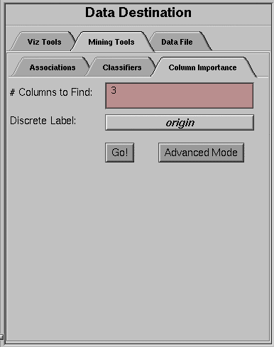
Column Importance (Figure 11-1) determines how important various columns are in discriminating the different values of the label column you choose. You might, for example, want to find out the best three columns for discriminating the label good credit risk so you can choose them for the Scatter Visualizer. When you select the label and click Go!, a popup window appears with the three columns that are the best three discriminators. A measure called “purity” (a number from 0 to 100) informs you how well the columns discriminate the different labels. Adding more columns can only increase the purity.
There are two modes of column importance:
Simple Mode
To invoke the Simple mode, choose a discrete label from the popup menu, and specify the number of columns you want to see, then click Go!.
Advanced Mode
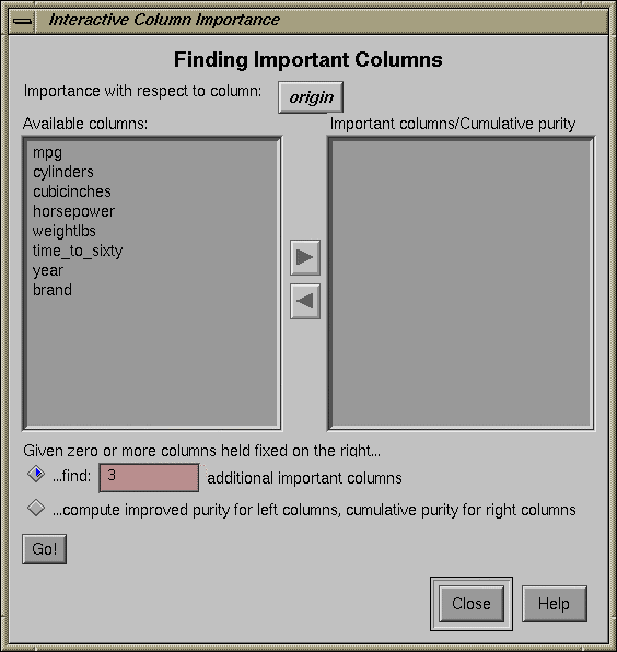
Advanced mode lets you control the choice of columns. To enter Advanced mode, click Advanced Mode in the Column Importance panel. A dialog box appears, as shown in Figure 11-2. The dialog box contains two lists of column names: The left list contains the available attributes and the right list contains attributes chosen as important (by either the user or the column importance algorithm).
Advanced mode can work two different ways: finding several new important attributes or ranking available attributes.
Finding Several Important Attributes
To enter this submode, click the first of the two radio buttons at the bottom of the dialog (...find [number] additional important attributes). If you click Go! with no further changes, the effect is the same as if you were in Simple mode, finding the specified number of important columns and automatically moving them to the right column. Near each column, the cumulative purity is given (that is, the purity of all the columns up to and including the one on the line. More attributes can only increase the purity.
Alternatively, by moving column names from the left list to the right list, you can prespecify columns that you want included and let the system add more. For example, to select the cylinders column and let the system find three more columns, click the cylinders column name, then click the right arrow between the lists.
Clicking Go! lets you see the cumulative purity of each column, together with the previous ones in the list. A purity of 100 means that using the given columns, you can perfectly discriminate the different label values in the dataset.
Ranking Available Attributes
Advanced mode also lets you compute the change in purity that each column would add to all those that were already marked important, that is, they are in the list on the right. For example, you might move cylinders to the list on the right, and then ask the system to compute the incremental improvement in purity that each column remaining in the left column would yield. The cumulative purity is computed for columns on the right.
To enter this submode, click the second of the two radio buttons at the bottom of the dialog (...compute improved purity for attributes on the left.). This submode permits fine control over the process. If two columns are ranked very closely, you might prefer one over the other (for example, because it is cheaper to gather, more reliable, or easier to understand).
Note that with other columns, the importance of features varies from their ranking alone. For example, while net-income might be a good column individually, it might not be as important together with salary because they are likely to be highly correlated. The best set of three columns is not necessarily composed of the columns that rank highest individually. If two columns give the income in dollars and in another currency, they are ranked equally alone; however, once one of them is chosen, the other adds no discriminatory power to the set of best features.
Column selection is useful for finding the best three axes for the Scatter Visualizer, as well as for finding a good discriminatory hierarchy (hierarchy that separates different label values) for the Tree Visualizer when you select the label to be the key used in the Tree Visualizer.
All floating point values (doubles or floats) are prediscretized using the automatic discretization (see Chapter 3, “The Tool Manager”). If a column has no value given to it in the left list, the algorithm did not consider it; this is because it either had a single value (for example, when it is discretized into one interval), or the number of records that it would separate are not statistically significant.
This section describes the differences among Column Importance, the importance ranking chosen by the Evidence Inducer, and the splits chosen by the Decision Tree Inducer. As Column Importance uses all of the data, these descriptions assume that you are running the inducers in “Classifier Only” mode, so that the inducers are using all of the data as well.
The column importance algorithm and the Evidence Inducer discretize all continuous attributes using the automatic discretization algorithm (the same algorithm that is applied in automatic binning in the Tool Manager). The decision tree algorithm does not pre-discretize attributes (columns) and finds thresholds as the tree is built.
The main advantage of the automatic discretization is that it discretizes the continuous range into several intervals at once, while the decision tree makes only binary splits.
The main advantage of the decision tree algorithm is that it discretizes subsets of the data (those that reach a specific node where a test is done). Thus the discretization is “local” to those records as opposed to a “global” discretization.
The Evidence Inducer and Column Importance rank attributes based on “mutual information” as the purity measure. The Decision Tree Inducer defaults to “normalized mutual information,” which penalizes multi-way splits (see the description of splitting criterion in “Decision Tree Inducer Options”). Thus, the Decision Tree Inducer prefers an attribute with few values over attributes with many values. The default for decision trees can be changed to “mutual information.”
The Evidence Inducer ranks each attribute independently. If several attributes are highly correlated, they have similar ranking. If you use the Advanced mode from Column Importance, the “...compute improved purity” option without any attributes chosen as important (that is, moved to the list on the right), the attribute ranking shown matches the sort order chosen by the Evidence Inducer.
Column Importance and the Decision Tree Inducer both provide more powerful importance capability than the Evidence Inducer. Both choose an importance ranking with respect to other attributes. In Column Importance, attributes are judged as important relative to the set of attributes in the list on the right. If two attributes are highly correlated and one is chosen, the other does not rank very highly. Similarly, in a decision tree, important attributes are chosen with respect to attributes on the path to the root node.
Decision trees provide the most flexible importance ranking because different attributes can be chosen at different subtrees. For example, one attribute can be chosen for the left child of the root and another for the right child of the root. With column importance, a single attribute must be chosen for all combinations of the previously chosen attributes. For some visualizations, such as the Scatter Visualizer, the Column Importance feature is most appropriate because you cannot represent a tree structure on the axes, yet you want to find a set of attributes that together give the most information.