This chapter provides a cursory introduction to classifiers and the algorithms that build them, called inducers. MineSet provides two inducer-classifier pairs:
Decision Tree
Evidence
The information in this chapter is equally applicable to either of these classifiers. Detailed descriptions of the MineSet inducers and classifiers are provided in Chapter 9, “Inducing and Visualizing the Decision Tree Classifier,” and Chapter 10, “Inducing and Visualizing the Evidence Classifier.”
A classifier predicts one attribute of a set of data given several other attributes. For example, if you have a database of iris flowers, a classifier can be built to predict the type of iris (iris-setosa, iris-versicolor, or iris-virginica) given the petal length, petal width, sepal length, and sepal width. The attribute being predicted (in this case, the type of iris) is called the label, and the attributes used for prediction are called the descriptive attributes.
MineSet can build a classifier automatically from a training set. This training set consists of records in the database for which the label has been determined, based on the descriptive attributes. For example, you supply a database table with one column for each descriptive attribute (such as petal length, petal width, sepal length, and sepal width) and one column for the label (iris-setosa, iris-versicolor, or iris-virginica). An algorithm that automatically builds a classifier from a training set is called an inducer.
When a classifier is generated, MineSet also generates a visualization that can help you understand how the classifier operates. This visualization can also provide valuable insight into the data itself.
Once a classifier is generated, it can be used to classify additional records not in the training set. These records need not contain the label attribute, since this value is predicted by the classifier.
 | Note: See Appendix I for a list of further readings about classifiers as well as acknowledgements for the datasets used in MineSet sample files. |
Figure 8-1 shows the decision tree generated by the Decision Tree inducer for the example mentioned above.
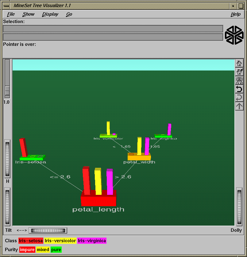
To understand how the Decision Tree classifier assigns a label to each record, look at the attributes tested at the nodes and the values on the connecting lines. In the decision tree shown in Figure 8-1, the first test (at the root of the tree) is for petal length. There are two branches from this root. If the petal length is ≤ 2.6, the left branch is taken; otherwise, the right branch is taken. The process is repeated until a leaf (final node) is reached. The leaf is labeled with the predicted class. The leaf represents a rule that is the conjunction of all tests from the root to the leaf. For example, the leaf labeled Iris-Virginica matches the rule
petal_length >2.6 and petal_width >1.65 implies iris_type = iris-virginica
Figure 8-2 shows the evidence information generated by the evidence inducer.
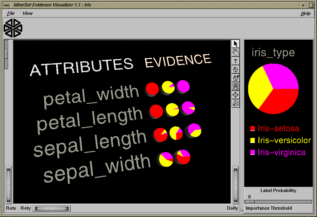
The right window of the screen shows the distribution of the classes in the training set. The left side shows rows of pie charts, one for each attribute. For every value of an attribute in the data, there is one pie chart matching it in the row for the attribute. Given a record with an attribute value corresponding to a pie chart, the pie chart represents how much evidence the classifier “adds” to each possible label value. For example, in Figure 8-2, a record with petal_width 1.2 (matching the second pie chart in the first row) adds much evidence for the iris-versicolor label value, little evidence for the iris-virginica label value, and no evidence for the iris-setosa label value. After evidence is accumulated from all the attributes (corresponding to one pie from every row), the label value with the most evidence is predicted.
An inducer is an algorithm that builds a classifier from a training set, which consists of records with labels. The training set is used by the inducer to “learn” how to construct the classifier, as shown in Figure 8-3.
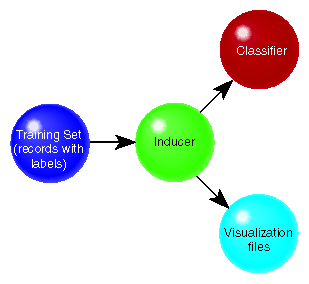
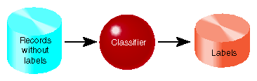
Once the classifier is built, its structure can be visualized or used to classify unlabeled records, as shown in Figure 8-3 and Figure 8-4.
Running inducers can be a CPU- and I/O-intensive process. For this reason, the MineSet inducers run on the server, rather than on your workstation (see Figure 8-5).
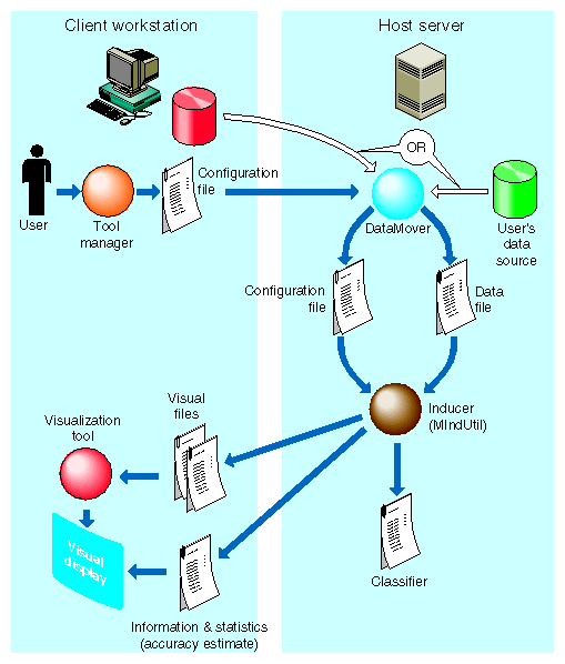
Inducers require a training set, which is a database table containing attributes, one of which is designated as the class label. The label attribute type must be discrete (binned values, character string values, or a few integers). The number of possible values for the label attribute should be small, preferably two or three values. The accuracy of the classifier is usually higher the fewer the number of label values. An example of this is the above-mentioned iris type attribute, which takes on one of three values (iris-setosa, iris-versicolor, or iris-virginica).
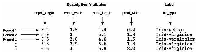
Figure 8-6 shows several records from a sample training set.
Once a classifier is built, it can classify new records as belonging to one of the classes (see Figure 8-4). These new records must be in a table that has the same attributes as the training set; however, the table need not contain the label attribute.
After building a classifier, you can apply it to records to predict the label (see “The Apply Classifier Button” in Chapter 3). For example, if you built a classifier for predicting iris_type, you can apply the classifier to records containing only the descriptive attributes, and a new column is added with the predicted iris type.
In a marketing campaign, for example, a training set can be generated by running the campaign at one city and generating label values according to the responses in the city. A classifier can then be induced and campaign mail can then be sent only to people who are labelled by the classifier as likely to respond, thus saving mailing costs.
As an example of using mining tools for data quality, after building a classifier you can apply it to the training set in order to identify records that are mislabeled by the classifier (use Classifier Only mode to train on the whole dataset). Such records could warrant closer investigation. Perhaps they are “noise,” or they might give special insights. If, for example, you have a decision tree for the iris dataset, by applying the classifier, you get a new column (iris_type_1) containing the predicted labels. You can then add a column that is defined as type int with the expression (iris_type != iris_type_1). The new column has a 1 whenever the classifier misclassifies, and a zero when it correctly classifies. Another alternative is to define the new column as a float with the expression (iris_type != iris_type_1) + 0.01. The Scatter Visualizer can then be used with the original label mapped to color, and this new column mapped to size. Incorrect predictions are shown as big cubes; correct predictions are shown as small cubes.
When a classifier is built, it is useful to know how well you can expect it to perform in the future (how accurate its classification will be). Factors affecting classification accuracy include the following:
The number of records available in the training set.
Since the inducer must learn from the training set, the larger the training set, the more reliable the classifier should be; however, the larger the training set, the longer it takes the inducer to build a classifier. The improvement to the accuracy decreases as the size of the training set increases (this is a case of diminishing returns).
The number of attributes.
More attributes mean more combinations for the inducer to compute, making the problem more difficult for the inducer and requiring more time. Note that sometimes random correlations can lead the inducer astray; consequently, it might build less accurate classifiers (technically, this is known as “overfitting”). If an attribute is irrelevant to the task, remove it from the training set (this can be done using the Tool Manager).
The information in the attributes.
Sometimes there is not enough information in the attributes to correctly predict the label with high accuracy (for example, trying to determine someone's salary based on their eye color). Adding other attributes (such as profession, hours per week, and age) might increase the accuracy.
The distribution of future unlabeled records.
If future records come from a distribution different from that of the training set, the accuracy will probably be low. For example, if you build a classifier to predict something from a training set containing family cars, it may not be useful to classify records containing many sport cars because the distribution of attribute values can be very different.
The two common methods for estimating the accuracy of a classifier are described below. Both of these assume that future records will be sampled from the same distribution as the training set.
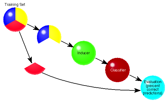
Holdout: A portion of the records (commonly two-thirds) is used as the training set, while the rest is kept as a test set. The inducer is shown only two-thirds of the data and builds a classifier. The test set is then classified using the induced classifier, and the accuracy on this test set is the estimated accuracy. Figure 8-7 shows this accuracy estimation method.
This method is fast, but since it uses only two-thirds of the data for building the classifier, it does not make efficient use of the data for learning. If all the data were used, it is possible that a more accurate classifier could be built.
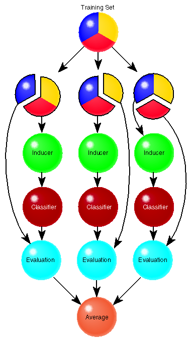
Cross-validation: The data is split into k mutually exclusive subsets (folds) of approximately equal size. The inducer is trained and tested k times; each time, it is trained on all the data minus a different fold, then tested on that heldout fold. The estimated accuracy is then the average of the accuracies obtained. Figure 8-8 shows cross-validation with k=3 (note that the default value is k=10).
Cross-validation can be repeated multiple times (t). For a t times k-fold cross-validation, k*t classifiers are built and evaluated. This means the time for cross-validation is k*t times longer. By default, k=10 and t=1, so cross-validation takes approximately 10 times longer than building a single classifier.
Increasing the number of repetitions (t) increases the running time and improves the accuracy estimate and the corresponding confidence interval.
You can increase or decrease k. Reducing it to 3 or 5 shortens the running time; however, estimates are likely to be biased pessimistically because of the smaller training set sizes. You can increase k, but this is recommended only for very small datasets.
Generally, a holdout estimate should be used at the exploratory stage, as well as on very large datasets. Cross-validation should be used for the final classifier building phase, as well as on small datasets.
There are three modes for running an inducer (shown in Figure 8-9).
Classifier and Accuracy
Classifier Only
Estimate Accuracy
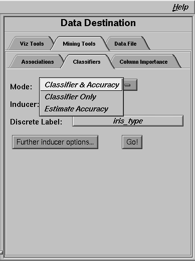
The Classifier and Accuracy mode uses a holdout method to build a classifier: a random portion of the data is used for training (commonly two-thirds) and the rest for testing. This holdout proportion can be set in Further Inducer Options (see “Accuracy Estimation”). This method is the default mode and is recommended for initial explorations. It is fast and provides an accuracy estimate.
The Classifier Only mode uses all the data to build the classifier. There is no accuracy estimation. Use this mode when there is little data or when you build the final classifier.
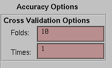
The Estimate Accuracy mode does not build a classifier, but assesses the accuracy of a classifier that would be built if all the data were used (as with Classifier Only mode). Estimate Accuracy uses cross-validation, resulting in long running times. Cross-validation splits the data into k folds (commonly 10) and builds k classifiers. The process can be repeated multiple times to increase the reliability of the estimate. You can set the number k and the number of times in Further Inducer Options, as explained in “Accuracy Options for Inducers” below.
Use this method when there is little data (less than 1,000 records), or when a classifier is built from the full dataset using the Classifier Only option and you need a final accuracy estimate.
The following options are available to fine tune the accuracy estimation for the inducers. The Accuracy Options available to you depend on the mode you have chosen.
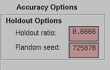
In both Classifier & Accuracy and Estimate Accuracy, you can see a random seed that determines how the data is split into training and testing sets. Changing the random seed causes a different split of the data into training and test sets. If the accuracy estimate varies appreciably, the induction process is not stable.
In Classifier & Accuracy (see Figure 8-10), you can set the Holdout Ratio of records to keep as the training set. This defaults to 0.6666 (two-thirds). The rest of the records are used for assessing the accuracy.
In Estimate Accuracy (see Figure 8-11), you can set the number of folds in cross validation and the number of times to repeat the process.
Once you have specified the Classification Options, click OK to have these options take effect and to return to the Data Destination panel. To return to the Data Destination panel without having changes to the options take effect, click Cancel.
After you press Go! in the Data Destination panel, an information and statistics popup appears (unless you specified Classifier Only mode, in which case only the visualization appears). It displays specific information for the induced classifier. For example, for decision trees it shows the number of nodes, the number of leaves, and the depth of the decision tree (Figure 8-12). This information is saved automatically on your workstation under the session file name with a -dt.out or -eviviz.out extension, depending on whether a decision tree inducer or an evidence inducer was executed. If you specified the Classifier & Accuracy or the Classifier Only mode, the Tree Visualizer is invoked automatically.
The information above the results line are “dribble” information to show progress.
For Classifier & Accuracy, the first series of dots represent reading the file, then information about the classifier build progress is shown, then the test set classification progress is shown.
For Classifier Only mode, there is no test set classification phase.
For Estimate Accuracy, the times and folds are shown.
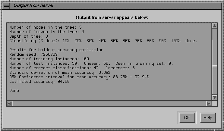
When you have selected the Classifier & Accuracy mode, the Information and Statistics popup window contains the following information:
The random seed used to split the data into training and test sets.
The number of records used for training the inducer.
The number of records used for evaluating the resulting classifier; of the test records, how many were seen during training, excluding the label attribute. It is possible to have duplicate records (“seen”) in a dataset; some records can be in both the training and test set. A large value of seen records indicates that there are many duplicate records. If their labels are contradictory, it may be impossible to achieve high accuracy without adding more attributes to the dataset.
The number of correct and incorrect predictions made.
The standard deviation of the estimated accuracy.
A 95% confidence interval for the mean accuracy. This is the appropriate range of accuracy you can expect from the classifier if the data comes from the same distribution. Technically, this uses a more accurate formula than the two-standard deviation rule usually applied in statistics.
The estimated accuracy.
When you have selected the Estimate Accuracy mode, the Information and Statistics popup window contains the following information:
The number of cross-validation folds and times.
The random seed.
The estimated accuracy with standard deviation.
The 95% confidence interval.
The following subsections describe how to set special options and the limitations of the inducers.
When the Tool Manager runs an inducer on the server (the MIndUtil program), it passes certain options to the inducers. Not all options are controlled through the Tool Manager GUI. Those options not controlled by Tool Manager take on their default values and can be overridden by setting them in a special file, called .mineset-classopt. Tool Manager prepends this file to the options sent. The file is optional. Tool Manager looks for it first in the current directory, then in your home directory. See Appendix E, “Command-Line Interface to MIndUtil: Classifiers, Discretization, Column Importance, and File Conversions” for more details about the options.
The file should contain one line per option, in the following format:
<OPTION>=<value> |
For example, the special option LOGLEVEL increases the amount of information shown during the induction process. The default of zero shows very little information. Level 1 shows other options and slightly more information. Level 2 and higher show large amounts of information about the induction process. These levels are appropriate only if you have a firm understanding of the induction process. (See Appendix I, “Further Reading and Acknowledgments.”)
Two limits and their respective options are as follows:
Discrete attributes are ignored if they have more than 50 values. Discrete attributes with many values are usually inappropriate for classification. For example, first names and street addresses are unlikely to form predictive patterns.
To speed up the induction process, attributes with over 50 values are ignored.
You can override this value by setting MAX_ATTR_VALS to a higher number. For example, your .mineset-classopt file could contain the line
MAX_ATTR_VALS=100
Discrete labels with over 25 values are not allowed by default. Automatically induced classifiers are rarely appropriate for predicting one of a large number of label values. You should limit the label to a few values (preferably two or three). You can override this default limit by setting the option MAX_LABEL_VALS to a higher value in your .mineset-classopt file.
There are three further limitations:
Floating point numbers are read into MIndUtil as floats (4 bytes) even if they are represented as doubles (8 bytes) in the database or ASCII file. This limits the precision and magnitude of the representations allowed.
Attributes of type arrays are always ignored.
Dates are considered strings. Unless there are few dates, such attributes are usually ignored because of the limit on discrete attributes. You should bin dates before running an inducer.