This chapter describes how to use NetCollect, NetPack, and NetAccount to collect network traffic data and produce reports that show an accounting of network usage. You can collect information such as the total number of packets transmitted by a particular protocol. You can also find the nodes that have transmitted the most packets and bytes.
Because you can use NetCollect to collect data for days, weeks, and months, you will be able to identify the nodes that most heavily use the network as well as identify trends in network use. And because NetCollect offers the potential to collect a large amount of data, you can pack (condense) the data with NetPack so it doesn't use as much disk space. You can produce reports from this data with NetAccount.
By reviewing the reports of network traffic, you can:
observe patterns of network use over a period of time
plan for network expansion by locating nodes that cause bottlenecks
track network use for accounting purposes
In addition to generating reports, you can also display and analyze the reports with a database or spreadsheet such as Wingz™. For information on Wingz, refer to the Wingz User's Guide.
This chapter explains how to:
collect data with NetCollect
combine data files created by NetCollect with NetPack
generate traffic reports with NetAccount
In addition, examples are provided. For complete information on NetCollect, NetPack, and NetAccount command line options, see the netcollect(1M), netpack(1M), and netaccount(1M) manual pages in Appendix F, “NetVisualyzer Manual Pages.”
 | Note: You must have authorization to use NetCollect. See “Authorizing NetVisualyzer Users for Snooping” in Chapter 1 and Appendix B, “Authorization Reference,” for details. |
To collect network traffic statistics, click the netcollect icon in the netvis directory view or enter:
netcollect & |
You can optionally enter the ampersand (&) to make the collection process run in the background. When a process runs in the background, that process's identification number (PID) is displayed on the screen. For example:
[1] 43258 |
You can use the number, 43258, to stop (by using the kill(1) command) the netcollect process. Or you can use the killall(1M) command. For example:
kill 43258 |
or
killall netcollect |
Until you kill netcollect, the data is collected from your workstation's default interface (for example, an Ethernet interface, ec0). Data is stored by default in files in a predefined directory structure in the current directory. The directory structure and file names are shown in Figure 7-1.
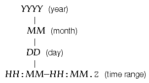
The files in the DD directory are named by using the starting and ending time of the sample interval. Hours are specified using a 24-hour clock. The file names end in .Z, indicating that they are compressed files.
The default sample interval is 1 hour. The first sample interval is adjusted, if necessary, so that the second and subsequent sample intervals begin at the start of the hour. For example, data collected starting at 10:00 a.m. is stored as:
10:00–10:59.Z |
Data collected beginning at 10:35 a.m. is stored in the file:
10:35–10:59.Z |
If a sample interval is not completed, a file is not generated.
For example, suppose you collect files daily in 1-hour intervals beginning at 9:30 a.m. and stopping at 18:30 (6:30 p.m.). You invoke NetCollect while in the directory named /usr/spool/netvis. Files produced by NetCollect on June 16, 1992 are stored in the directory named /usr/spool/netvis/1992/06/16.
A listing of the directory looks like this:
09:30-09:59.Z 12:00-12:59.Z 15:00-15:59.Z 10:00-10:59.Z 13:00-13:59.Z 16:00-16:59.Z 11:00-11:59.Z 14:00-14:59.Z 17:00-17:59.Z |
Notice that there is no file for the period of 6:00 p.m. to 6:30 p.m. No file was created because the sample interval of 6:00 p.m. to 7:00 p.m. wasn't completed.
A sample report later in this chapter shows a portion of the data stored in one of NetCollect's data files. The report was generated by NetAccount. Notice the level of detail and the amount of data in this file. Be aware of the amount of disk space used by the NetCollect files. To free up disk space, it's best to periodically archive and remove the files.
You may want to create a shell script to collect the data and take advantage of cron(1M) to start and stop collection, pack the files, or produce reports of the data. Refer to the /usr/people/4Dgifts/examples/netvis directory for an example of a script you can use to pack files.
The next sections explain how to use the options to NetCollect.
To collect data from an interface other than the default, use the –i option. For example, suppose you want to collect data from a Data Station that has the additional EFast Ethernet board (fxp0). To do this, type:
netcollect -i fxp0 & |
It's recommended that you collect data locally. However, you may want to capture packets from the default interface on a remote Data Station. For example, to collect data from the default interface of a Data Station named outback, type:
netcollect -i outback: & |
Notice that you do not have to type the default interface. If you want to collect data from a remote Data Station's interface that is not the default, you must specify it. For example, assume outback has the additional EFast Ethernet board installed. To capture from this interface, type:
netcollect -i outback:fxp0 & |
Use NetPack to coalesce data files obtained from NetCollect. When files are packed, all the data from the NetCollect files you specify is added together; therefore, you lose each individual file's time resolution. For example, you may want to pack all the files for a week; thus you will have only one data file for the week. Or you may want to pack a day's worth of files (all the files collected daily between 08:00 and 18:00) into one data file.
To pack files, double-click the netpack icon in the netvis directory view or give the command using the syntax:
netpack datafile1 datafile2 ... datafilen |
where each datafile is a file produced by NetCollect. When you double-click the icon, a Launch Command window appears. Complete the command line using the syntax shown above.
The following example packs NetCollect data files produced on June 16 from 09:00 to 18:00. First, change to the directory that contains the files:
cd /usr/spool/netvis/1992/06/16 |
You can use the wildcard character (*) to pack all the files:
netpack * & |
or you can specify individual file names:
netpack 09:00-09:59 10:00-10:59 11:00-11:59 12:00-12:59 \ 13:00-13:59 14:00-14:59 15:00-15:59 16:00-16:59 & |
Notice that you do not have to specify a file in which to put the packed files. NetPack automatically creates the file for you. When it packs files, NetPack reads each data file in the list and merges the data into a single file. The newly created file is then written to the directory structure used by NetCollect.
By default, the current directory is checked to see if it contains a year directory or is part of a data directory structure. If it finds a data directory structure, that structure is used; otherwise, a directory structure is created in the current directory.
Files packed from the previous NetPack command are put in the directory /usr/spool/netvis/1992/06/16 in the file:
09:00-16:59.Z |
If the file spans 2 days, it is placed in the MM directory and is named appropriately. For example:
04@17:00–05@08:59.Z |
If the file spans months, it is placed in the YYYY directory. For example:
01.01@00:00–12.31@23:59.Z |
If the file spans years, it is placed in the top-level directory. For example:
1990.01.01@00:00–1992.12.31@23:59.Z |
The –r option allows you to remove the original NetCollect data files after they are packed together. For example:
netpack -r datafile1 datafile2 |
packs datafile1 and datafile2 together and then removes them. Once you delete a NetCollect data file, you cannot retrieve that file's data because that data was merged with the other packed files' data.
After collecting the data, use NetAccount to generate a report of the network traffic. You can generate the report from files produced by either NetCollect or NetPack.
To generate a report, double-click the netaccount icon in the netvis directory view or enter:
netaccount datafile > reportfile |
where datafile is either a NetCollect or NetPack file, and reportfile is the file in which to write the report. Output appears on the screen if you do not redirect it (by using the > character) to a file. When you double-click the icon, a Launch Command window appears. Complete the command line using the syntax shown above.
For example, to see the traffic statistics in the file 09:00-16:59.Z produced by NetPack, change to the /usr/spool/netvis/1992/06/16 directory and type:
netaccount 09:00-16:59.Z |
By default, the report ranks the top five nodes in order of most packets and most bytes, summarizes nodes having 25% or more of the packets of any protocol and nodes having 25% or more of the bytes of any protocol, and produces counts of total bytes and total packets by protocol. By default, a report contains the following six sections:
Traffic Summary
Total
Source Ranking
Source Summary
Destination Ranking
Destination Summary
Each section of the report is described below and a portion of that section of a report is shown. The report used in these examples was based on data that was collected over intervals of two minutes. The NetAccount command with no options was used to create the report.
The Traffic Summary section lists the network segment from which the data was collected and the Data Station that collected the data. The date and time the data was collected is listed, too. For example, the Traffic Summary section is:
               ==========   Traffic Summary   ==========

Network:        b9l-pubs(192.26.79.0)
Collector:      yeti.wpd.sgi.com(192.26.79.6)
From:           Tue Jun 16 09:46:26 1992 PDT
To:             Tue Jun 16 10:29:59 1992 PDT
|
The Total list shows the total number of packets and bytes transmitted in each protocol during the report period. For example, part of the Total section might look like this:
            ----------        Total        ----------

Protocol       Packets                            Bytes

ether           193572                         34470280
arp                 78                             4680
arpip               78                             4680
ip              193494                         34465600
icmp              5815                           549066
igmp               102                             6120
tcp              33071                          9941938
udp             151672                         20120828
|
The Source Ranking part of the report is organized by protocol. For each protocol, NetAccount ranks the top source nodes first by the number of packets sent and second by the number of bytes sent. Nodes are listed by name (if known), IP address, and physical address. The next line after each node contains the number of packets sent, the percentage of the packets of that protocol sent by that node, the number of bytes sent, and the percentage of the bytes of that protocol sent by that node. For example, part of the Source Ranking section looks like this:
                ----------   Source Ranking    ----------
                                 Top 5

ether
  Ranked by packets:
    1. paganini.wpd.sgi.com(192.26.79.1)[8:0:69:2:29:38/SGI]
                     65221 [ 33.69%]                6864078 [ 19.91%]
    2. eno.wpd.sgi.com(192.26.79.24)[8:0:69:6:59:22/SGI]
                     44378 [ 22.93%]                7037132 [ 20.42%]
...

  Ranked by bytes:
    1. eno.wpd.sgi.com(192.26.79.24)[8:0:69:6:59:22/SGI]
                     44378 [ 22.93%]                7037132 [ 20.42%]
    2. paganini.wpd.sgi.com(192.26.79.1)[8:0:69:2:29:38/SGI]
                     65221 [ 33.69%]                6864078 [ 19.91%]
...
|
The Source Summary list is organized by source nodes. Each source node that accounts for at least 25% percent, by default, of the packets or bytes of any protocol is listed (sorted by address). For each source node, each protocol used is listed. For each protocol, the number of packets sent, the percentage of all packets of that protocol sent by this node, the number of bytes sent, and the percentage of all bytes of that protocol sent by this node is listed. For example, part of the Source Summary section looks like this:
                ----------   Source Summary    ----------
                Minimum 25% of protocol packets or bytes

mantis.wpd.sgi.com(192.26.79.15)[8:0:69:2:29:23/SGI]
  total:
    ether             2662 [  1.38%]                 260770 [  0.76%]
    ip                2662 [  1.38%]                 260770 [  0.76%]
    icmp              2629 [ 45.21%]                 257246 [ 46.85%]
    igmp                 1 [  0.98%]                     60 [  0.98%]
    udp                 32 [  0.02%]                   3464 [  0.02%]
    tsp                 11 [  1.92%]                   1298 [  1.92%]

eno.wpd.sgi.com(192.26.79.24)[8:0:69:6:59:22/SGI]
  total:
    ether            44378 [ 22.93%]                7037132 [ 20.42%]
    arp                  1 [  1.28%]                     60 [  1.28%]
    arpip                1 [  1.28%]                     60 [  1.28%]
    ip               44377 [ 22.93%]                7037072 [ 20.42%]
    icmp                11 [  0.19%]                    682 [  0.12%]
    tcp               9650 [ 29.18%]                2574358 [ 25.89%]
    udp              34716 [ 22.89%]                4462032 [ 22.18%]
    dns                  4 [  0.56%]                    296 [  0.35%]
    sunrpc              25 [  0.12%]                   4298 [  0.09%]
    nfs                  9 [  0.04%]                   1322 [  0.02%]
    pmap                 8 [  3.33%]                    784 [  2.97%]
    telnet               1 [100.00%]                     60 [100.00%]
    tsp                 11 [  1.92%]                   1298 [  1.92%]
    rcp               3058 [ 51.80%]                2176609 [ 49.41%]
|
The Destination Ranking part of the report is organized by protocol. For each protocol, the top destination nodes are ranked first by the number of packets received and second by the number of bytes received. Nodes are listed by name (if known), IP address, and physical address. The next line after each node contains the number of packets received, the percentage of the packets of that protocol received by that node, the number of bytes received, and the percentage of the bytes of that protocol received by that node. For example, part of the Destination Ranking section looks like this:
                ---------- Destination Ranking ----------
                                 Top 5

ether
  Ranked by packets:
    1. paganini.wpd.sgi.com(192.26.79.1)[8:0:69:2:29:38/SGI]
                     64679 [ 33.41%]                8252867 [ 23.94%]
    2. eno.wpd.sgi.com(192.26.79.24)[8:0:69:6:59:22/SGI]
                     43272 [ 22.35%]                6137764 [ 17.81%]
...

  Ranked by bytes:
    1. paganini.wpd.sgi.com(192.26.79.1)[8:0:69:2:29:38/SGI]
                     64679 [ 33.41%]                8252867 [ 23.94%]
    2. eno.wpd.sgi.com(192.26.79.24)[8:0:69:6:59:22/SGI]
                     43272 [ 22.35%]                6137764 [ 17.81%]
...
|
The Destination Summary list is organized by destination nodes. Each destination node that accounts for at least 25% percent, by default, of the packets or bytes of any protocol is listed (sorted by address). For each destination node, each protocol used is listed. For each protocol, the number of packets received, the percentage of all packets of that protocol received by this node, the number of bytes received, and the percentage of all bytes of that protocol received by this node is listed. For example, part of the Destination Summary section looks like this:
                ---------- Destination Summary ----------
                Minimum 25% of protocol packets or bytes

paganini.wpd.sgi.com(192.26.79.1)[8:0:69:2:29:38/SGI]
  total:
    ether            64679 [ 33.41%]                8252867 [ 23.94%]
    ip               64679 [ 33.43%]                8252867 [ 23.95%]
    icmp               281 [  4.83%]                  17422 [  3.17%]
    udp              64398 [ 42.46%]                8235445 [ 40.93%]
    dns                211 [ 29.63%]                  35275 [ 41.68%]
    sunrpc               8 [  0.04%]                    608 [  0.01%]
    pmap                 2 [  0.83%]                    140 [  0.53%]
    tsp                280 [ 48.78%]                  33040 [ 48.78%]

calliope.wpd.sgi.com(192.26.79.9)[2:cf:1f:11:39:75/CMC]
  total:
    ether             3995 [  2.06%]                 468118 [  1.36%]
    ip                3995 [  2.06%]                 468118 [  1.36%]
    icmp              2629 [ 45.21%]                 257246 [ 46.85%]
    udp               1366 [  0.90%]                 210872 [  1.05%]
    sunrpc            1332 [  6.15%]                 207504 [  4.28%]
    nfs               1326 [  5.52%]                 206844 [  2.40%]
    pmap                 3 [  1.25%]                    294 [  1.11%]
    tsp                 11 [  1.92%]                   1298 [  1.92%]
|
The following sections contain examples for NetCollect, NetPack, and NetAccount—planning prior to running NetCollect, producing a report of a specific protocol, collecting data in a distributed environment, and producing verbose reports.
Because you are collecting large amounts of data (about 120K per hour for NetCollect), you should consider the amount of disk space on your system. Examples of other questions to consider are:
What time period do you want to use when collecting the data—how many hours (for example, between working hours of 8:00 a.m. to 5:00 p.m. or 24 hours a day), and on which days (for example, 5 working days or 7 days)?
What sample interval do you want to use when collecting the data—how many minutes' worth of data do you want in each file (the default is 60 minutes)?
How often do you want to pack the files—every day, week, or month?
How do you want to pack the files—pack the entire day's files into one file, or pack all files within a specific time interval into one file?
How long do you want to keep the original files after you pack them?
How often do you want to produce reports?
What files do you want to archive?
When do you want to remove the data, packed data, and report files?
For information on administrative tasks, such as how to determine disk space and how to archive and back up files, see the Personal System Administration Guide.
The –p option of the netaccount command allows you to produce a report of a specific protocol's network traffic. The syntax is:
netaccount -p protocol datafile |
where protocol is the protocol name and datafile is a NetCollect or NetPack file. You can specify more than one protocol. For example, to produce a report of NFS and TCP traffic that occurred between 9:00 a.m. and 9:59 a.m., type:
netaccount -p nfs -p tcp 09:00-09:59 |
Just as with NetLook, NetGraph, Analyzer, and NetTop, you can take advantage of NetCollect, NetPack, and NetAccount to monitor networks in a distributed environment. To use NetCollect, NetPack, and NetAccount in a distributed environment, connect a Data Station to every network segment. Each Data Station can collect data and generate accounting reports that can reside on the Data Station's disk.
To obtain data about remote nodes and ports, use the –v (verbose) option of the netaccount command. This option is cumulative; for example, –vv includes –v data and produces additional data. With no –v option, sources and destinations that are matched by IP address are shown. The additional information you get with –v options is:
| –v | Sources and destinations are matched by physical addresses. This provides different results from matching IP addresses when packets from one host travel through two routers. | |
| –vv | The sources and destinations are broken down: for each source, show statistics for each destination separately in the Source Summary; for each destination, show statistics for each source separately in the Destination Summary. | |
| –vvv | Break down the –vv information by port number. This shows individual packet transactions. |
First, look at a small part of the source summary produced without the –v option (or with the –v option, they are the same) for a node named bonnie.
                ----------   Source Summary    ----------
                Minimum 25% of protocol packets or bytes

bonnie.wpd.sgi.com(192.26.61.14)[8:0:69:2:1e:dc/SGI]
  total:
    ether           211494 [ 28.79%]              127948448 [ 34.55%]
    arp                  4 [  0.37%]                    240 [  0.37%]
    arpip                4 [  0.35%]                    240 [  0.35%]
    ip              211490 [ 28.85%]              127948208 [ 34.56%]
    igmp                 2 [  0.25%]                    120 [  0.13%]
    tcp              85787 [ 18.00%]                5147943 [  2.31%]
    udp              64957 [ 34.00%]               40140468 [ 64.84%]
    rip                180 [  3.51%]                  11880 [  0.59%]
    sunrpc           64777 [ 25.92%]               40128588 [ 35.10%]
    nfs             109413 [ 60.15%]              108771904 [ 87.53%]
    pmap                12 [  0.30%]                   1008 [  0.28%]
|
In this example, bonnie accounted for 211494 ether packets, which was 28.79% of all ether packets and 12794884 ether bytes, which was 34.55% of all ether bytes.
With the –vv option, the packets are broken out by destination. For example:
                ----------   Source Summary    ----------
                Minimum 25% of protocol packets or bytes

bonnie.wpd.sgi.com(192.26.61.14)[8:0:69:2:1e:dc/SGI]
          -> rains.wpd.sgi.com(192.26.61.4)[8:0:69:2:15:88/SGI]
    ether           209743 [ 28.55%] [ 99.17%]    127609232 [ 34.46%] [ 99.73%]
    ip              209743 [ 28.61%] [ 99.17%]    127609232 [ 34.47%] [ 99.74%]
    tcp              85754 [ 17.99%] [ 99.96%]      5145240 [  2.31%] [ 99.95%]
    udp              63292 [ 33.12%] [ 97.44%]     39871284 [ 64.40%] [ 99.33%]
    sunrpc           63292 [ 25.33%] [ 97.71%]     39871284 [ 34.88%] [ 99.36%]
    nfs             109211 [ 60.04%] [ 99.82%]    108736096 [ 87.50%] [ 99.97%]
          -> zoomer.wpd.sgi.com(192.26.61.9)[8:0:69:2:12:fc/SGI]
    ether                4 [  0.00%] [  0.00%]          474 [  0.00%] [  0.00%]
    arp                  1 [  0.09%] [ 25.00%]           60 [  0.09%] [ 25.00%]
    arpip                1 [  0.09%] [ 25.00%]           60 [  0.09%] [ 25.00%]
    ip                   3 [  0.00%] [  0.00%]          414 [  0.00%] [  0.00%]
    udp                  3 [  0.00%] [  0.00%]          414 [  0.00%] [  0.00%]
    sunrpc               3 [  0.00%] [  0.00%]          414 [  0.00%] [  0.00%]
    nfs                  2 [  0.00%] [  0.00%]          276 [  0.00%] [  0.00%]
|
In this example, packets from bonnie to rains accounted for 209743 ether packets, which is 28.55% of all ether packets and 99.17% of bonnie's ether packets.
The –vvv option additionally lists all ports that were accessed. The size of the report substantially increases the time it takes to generate the report. For example:
                ----------   Source Summary    ----------
                Minimum 25% of protocol packets or bytes

bonnie.wpd.sgi.com(192.26.61.14)[8:0:69:2:1e:dc/SGI]
     2049 -> rains.wpd.sgi.com(192.26.61.4)[8:0:69:2:15:88/SGI].1023
    ether            61490 [  8.37%] [ 29.07%]     39123088 [ 10.56%] [ 30.58%]
    ip               61490 [  8.39%] [ 29.07%]     39123088 [ 10.57%] [ 30.58%]
    udp              61490 [ 32.18%] [ 94.66%]     39123088 [ 63.19%] [ 97.47%]
    sunrpc           61490 [ 24.60%] [ 94.93%]     39123088 [ 34.22%] [ 97.49%]
    nfs              52617 [ 28.93%] [ 48.09%]     32456046 [ 26.12%] [ 29.84%]
     2049 -> zoomer.wpd.sgi.com(192.26.61.9)[8:0:69:2:12:fc/SGI].1023
    ether                3 [  0.00%] [  0.00%]          414 [  0.00%] [  0.00%]
    ip                   3 [  0.00%] [  0.00%]          414 [  0.00%] [  0.00%]
    udp                  3 [  0.00%] [  0.00%]          414 [  0.00%] [  0.00%]
    sunrpc               3 [  0.00%] [  0.00%]          414 [  0.00%] [  0.00%]
    nfs                  2 [  0.00%] [  0.00%]          276 [  0.00%] [  0.00%]
|
In this example, bonnie sent 61490 ether packets from its port 2049 to rains, which is 8.37% of all ether packets and 29.07% of bonnie's ether packets.