LAPACK is a public domain library of subroutines for solving dense linear algebra problems, including systems of linear equations, linear least squares problems, eigenvalue problems, and singular value decomposition problems. It has been designed for efficiency on high-performance computers.
LAPACK is the successor to LINPACK and EISPACK. It uses today's high-performance computers more efficiently than the older packages and it extends the functionality of these packages by including equilibration, iterative refinement, error bounds, and driver routines for linear systems. It also includes routines for computing and reordering the Schur factorization, and condition estimation routines for eigenvalue problems.
Performance issues are addressed by implementing the most computationally-intensive algorithms using the Level 2 and 3 Basic Linear Algebra Subprograms (BLAS). Because most of the BLAS were optimized in single and multiple-processor environments, these algorithms give near optimal performance.
All routines from LAPACK 3.0 are included in SCSL. This includes driver routines, computational routines, and auxiliary routines for solving linear systems, least squares problems, and eigenvalue and singular value problems. See the INTRO_LAPACK (3S) man page for details about the routines that are available in the current release of SCSL.
Online man pages are available for individual LAPACK subroutines. For example, to view a description of the calling sequence for the subroutine to perform the LU factorization of a real matrix, see the DGETRF(3S) man page. The user interface to all supported LAPACK routines is the same as the standard LAPACK interface.
Several enhancements improve the performance of the LAPACK routines on SGI systems. For example, the LU, Cholesky, and QR factorization routines are redesigned for better performance and scalability when running multiple processes.
Tuning parameters for the block algorithms provided in SCSL are set within the ILAENV LAPACK routine. ILAENV is an integer function subprogram that accepts information about the problem type and problem dimensions and returns a single integer parameter such as the optimal block size, the minimum block size for which a block algorithm should be used, or the crossover point (the problem size at which it becomes more efficient to switch to an unblocked algorithm). Setting tuning parameters occurs without user intervention, but users can call ILAENV directly to check the values to be used.
The name of each LAPACK routine is a coded specification of its function. All driver and computational routines have five or six character names of the form XYYZZ or XYYZZZ. The first letter, X, indicates the data type:
S: real
D: double precision
C: complex
Z: double complex
The next two letters, YY, indicate the type of matrix or the most signficant matrix type. Most of these two letter codes apply to both real and complex matrices, but some apply specifically to only one or the other. The following list shows all matrix types:
BD     BiDiagonal
     DI     Diagonal
     GB     General Band
     GE     GEneral (nonsymmetric)
     GG     General matrices, Generalized problem
     GT     General Tridiagonal
     HB     Hermitian Band (complex only)
     HE     HErmitian (possibly indefinite) (complex only)
     HG     Hessenberg matrix, Generalized problem
     HP     Hermitian Packed (possibly indefinite) (complex only)
     HS     upper HeSsenberg
     OP     Orthogonal Packed (real only)
     OR     ORthogonal (real only)
     PB     Positive definite Band (symmetric or Hermitian)
     PO     POsitive definite (symmetric or Hermitian)
     PP     Positive definite Packed (symmetric or Hermitian)
     PT     Positive definite Tridiagonal (symmetric or Hermitian)
     SB     Symmetric Band (real only)
     SP     Symmetric Packed (possibly indefinite)
     ST     Symmetric Tridiagonal
     SY     SYmmetric (possibly indefinite)
     TB     Triangular Band
     TG     Triangular matrices, Generalized problem
     TP     Triangular Packed
     TR     TRiangular
     TZ     TrapeZoidal
     UN     UNitary (complex only)
     UP     Unitary Packed (complex only)
|
The last letters, ZZ or ZZZ, indicate the computation performed. For example, TRF is a Triangular Factorization.
See the INTRO_LAPACK(3s) man page for details about the types of computations performed and a list of supported routines.
LAPACK routines can solve systems of linear equations, linear least squares problems, eigenvalue problems, and singular value problems. LAPACK routines can also handle many associated computations such as matrix factorizations and estimating condition numbers. Dense and banded matrices are provided for, but not general sparse matrices.
This subsection discusses the LAPACK routines for solving the following two basic problems:
Computing the unique solution to a linear system
 , where the coefficient matrix A
is dense, banded, triangular, or tridiagonal, and the matrix
B may contain one or more right-hand sides.
, where the coefficient matrix A
is dense, banded, triangular, or tridiagonal, and the matrix
B may contain one or more right-hand sides.Computing a least squares solution to an overdetermined system
 , where A is
  with
with  , or a minimum norm solution to an underdetermined system
  , where A is
  with
with  .
.
See “Solving Linear Systems”, and “Solving Least Squares Problems”, for a discussion of the software used to solve these problems. The orthogonal transformation routines described in “Solving Least Squares Problems”, also have application in eigenvalue and singular value computations.
There are three classes of LAPACK routines: LAPACK driver routines solve a complete problem; LAPACK computational routines perform one step of the computation; and LAPACK auxiliary routines perform certain subtask or low-lvel computation.
The driver routines generally call the computational routines to do their work, and offer a more convenient interface; therefore, LAPACK users are advised to use a driver routine if there is one that meets their requirements.
Man pages for both driver and computational routines are available with SCSL. A list of the auxiliary routines, with a brief description, can be found in the LAPACK User's Guide.
Finding the solution of a system of simulataneous linear equations is one of the most frequently encountered problems in scientific computing.
A linear system of equations (n equations with n unknowns) can be written as follows:
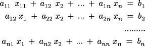
This system can also be written in the form  where A is a square matrix
of order n, b is
a given column vector of n components and
x is an unknown column vector of n
components.
where A is a square matrix
of order n, b is
a given column vector of n components and
x is an unknown column vector of n
components.
For example, the following linear equations:

can be written in matrix/vector notation as the following:
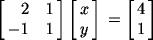
The solution to this system of equations is the set of vectors  that satisfy both equations. The physical interpretation
of this system of equations is that it represents two lines in the (
x,y) plane, which may intersect
in one point, no points (if they are parallel), or an infinite number
of points (if the two equations are multiples of each other).
that satisfy both equations. The physical interpretation
of this system of equations is that it represents two lines in the (
x,y) plane, which may intersect
in one point, no points (if they are parallel), or an infinite number
of points (if the two equations are multiples of each other).
To solve the system, it is helpful to simply the system as much as possible. A standard method for doing this (Gaussian elimination) is to use the following elementary operations:
interchange any two equations
multiply an equation by a nonzero constant
add a multiple of one equation to any other one
This reduces the system to a triangular form. The system obtained after each operation will be equivalent to the original system and therefore have the same solution.
For illustration consider the following system of linear equations:
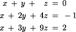
Subtract the first equation from the second equation and subtract the first equation from the third one. The result is the following system:
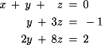
Note the first variable x no longer appears in the second or third equation. Similarly, the second variable y can be eliminated from the third equation by subtracting 2 times the second equation from the third equation to obtain the following:
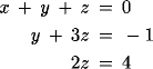
The resulting system is upper triangular and it can easily be deduced that:

To represent these steps in matrix form, let A=A1, A2, and A3 represent the matrices of the systems (Equation 3-4, Equation 3-5, Equation 3-6, respectively), for example:
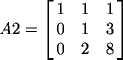
Then A2 is obtained from A1 by subtracting the first row from the second row and subtracting the first row from the third row. This means that A2 can be obtained by pre-multiplying A1 by a suitable matrix, and in this example, it is easy to verify that

that is:
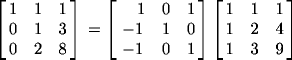
In a similar way

or
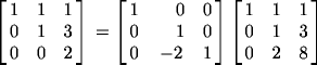
Combining Equation 3-9 and Equation 3-11 we have

Therefore, to solve the system Ax=b, we only need to calculate the following:

and solve the upper triangular system

Moreover, M1 and M2 are nonsingular matrices so:

Because M1 and M2 are unit lower triangular, so is the product of their inverses. Therefore, A can be written as the product of a lower triangular matrix L=M1-1 × M2-1 and an upper triangular matrix U=A3. Equation 3-16 becomes A=LU, which is the factorization of the coefficient matrix A.
The LAPACK routines for solving linear systems assume the system is already in a matrix form. The data type (real or complex), characteristics of the coefficient matrix (general or symmetric, and positive definite or indefinite if symmetric), and the storage format of the matrix (dense, band, or packed), determine the routines that should be used.
Most of the techniques in LAPACK are based on a matrix factorization as the first step. There are two main types of factorization forms:
explicit: The actual factors are returned. For example, the Cholesky factorization routine DPOTRF(3S), with UPLO = `L', returns a matrix L such that
 .
.factored form: The factorization is returned as a product of permutation matrices and triangular matrices that are low-rank modifications of the identity. For example, the diagonal pivoting factorization routine DSYTRF(3S), with UPLO = `L', computes a factorization of the following form:
where each
 is a rank-1 permutation, each
  is a rank-1 or rank-2 modification of the identity,
and D is a diagonal matrix with 1-by-1 and
2-by-2 diagonal blocks.
is a rank-1 or rank-2 modification of the identity,
and D is a diagonal matrix with 1-by-1 and
2-by-2 diagonal blocks.

Generally, users do not have to know the details of how the factorization is stored, because other LAPACK routines manipulate the factored form.
Regardless of the form of the factorization, it reduces the solution
phase to one that requires only permutations and the solution of triangular
systems. For example, the LU factorization of a general matrix,  , is used to solve for X in
the system of equations
, is used to solve for X in
the system of equations  by successively applying the inverses of
P, L, and U
to the right-hand side:
by successively applying the inverses of
P, L, and U
to the right-hand side:


In the last two steps, the inverse of the triangular factors is
not computed, but triangular systems of the form  and
and  are solved instead.
The following table lists the factorization forms for each of the factorization routines for real matrices. The factorization forms differ for DGETRF and DGBTRF, even though both compute an LU factorization with partial pivoting. You can also obtain the same factorizations through the LAPACK driver routines (for instance, DGESV or DGESVX).
Table 3-1. Factorization forms
Name | Form | Equation | Notes |
|---|---|---|---|
DGBTRF | Factored form | A = LU | L is a product of permutations and unit lower triangular matrices Li; Li differs from the identity matrix only in column i. |
DGTTRF | Factored form | A = LU | |
DGETRF | Explicit | A = PLU | |
DPBTRF | Explicit | A = LLT or A = UT U | |
DPOTRF | Explicit | A = LLT or A = UT U | |
DPPTRF | Explicit | A = LLT or A = UT U | |
DPTTRF | Explicit | A = LDLT or A = UT DU | |
DSPTRF | Factored form | A = LDLT or A = UDUT | L (or U) is a product of permutations and block unit lower (upper) triangular matrices Li (Ui); Li (Ui) differs from the identity matrix only in the one or two columns that correspond to the 1-by-1 or 2-by-2 diagonal block Di. |
DSYTRF | Factored form | A = LDLT or A = UDUT |
The
DGETRF subroutine performs an LU factorization with partial
pivoting ( ) as the first step in solving a general system of linear
equations
) as the first step in solving a general system of linear
equations  . If DGETRF is called with the following:
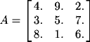
details of the factorization are returned, as follows:
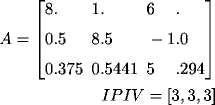
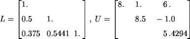
Matrices L and U are given explicitly in the lower and upper triangles, respectively, of A:
The IPIV vector specifies the row interchanges that were performed. IPIV(1)= 3 implies that the first and third rows were interchanged when factoring the first column; IPIV(2)= 3 implies that the second and third rows were interchanged when factoring the second column. In this case, IPIV(3) must be 3 because there are only three rows. Thus, the permutation matrix is the following:

Generally, the pivot information is used directly from IPIV without constructing matrix P.
Example 3-2. Symmetric indefinite matrix factorization
DSYTRF
factors a symmetric indefinite matrix A
into one of the forms  or
or  , where L and
U are lower triangular and upper triangular matrices, respectively,
in factored form, and D is a diagonal matrix
with 1-by-1 and 2-by-2 diagonal blocks. To illustrate this factorization,
choose a symmetric matrix that requires both 1-by-1 and 2-by-2 pivots:
, where L and
U are lower triangular and upper triangular matrices, respectively,
in factored form, and D is a diagonal matrix
with 1-by-1 and 2-by-2 diagonal blocks. To illustrate this factorization,
choose a symmetric matrix that requires both 1-by-1 and 2-by-2 pivots:
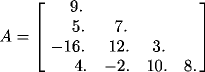
Only the lower triangle of A is specified because the matrix is symmetric, but you could have specified the upper triangle instead. The output from DSYTRF is the following:
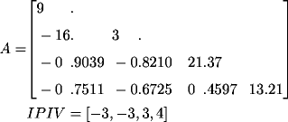
The signs of the indices in the IPIV vector indicate that a 2-by-2 pivot block was used for the first two columns, and 1-by-1 pivots were used for the third and fourth columns. Therefore, D must be the following:
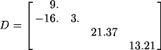
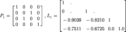
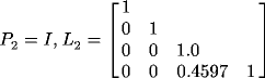
Matrix L is supplied in factored form
as  , where the parts of each
  that differ from the identity are stored in
A below their corresponding blocks
that differ from the identity are stored in
A below their corresponding blocks  :
:
The LAPACK routines always check the arguments on entry for incorrect values. If an illegal argument value is detected, the error-handling subroutine XERBLA is called. XERBLA prints a message similar to the following to standard error, and then it aborts:
** On entry to DGETRF parameter number 4 had an illegal value |
All other errors in the LAPACK routines are described by error codes returned in info, the last argument. The values returned in info are routine-specific, except for info = 0, which always means that the requested operation completed successfully.
For example, an error code of info >
0 from DGETRF means that one of the diagonal elements
of the factor U from the factorization  is exactly 0. This indicates that one of the rows of
A is a linear combination of the other rows, and the linear
system does not have a unique solution.
is exactly 0. This indicates that one of the rows of
A is a linear combination of the other rows, and the linear
system does not have a unique solution.
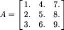
it returns
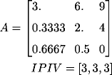
which corresponds to the factorization

On exit from DGETRF, info
= 3, indicating that U(3,3) is exactly 0. This
is not an error condition for the factorization because the factors that
were computed satisfy  , but the factorization cannot be used to solve the system.
In LAPACK, the solution step is generally separated
from the factorization. This allows the matrix factorization to be reused
if the same coefficient matrix appears in several systems of equations
with different right-hand sides. If the number of right-hand sides is
also large, it is often more efficient to separate the solve from the
factorization. The typical usage is found in the driver routine
DGESV, which solves a general system of equations  by using two subroutine calls, the first to factor the
matrix A and the second to solve the system,
using the factored form:
by using two subroutine calls, the first to factor the
matrix A and the second to solve the system,
using the factored form:
CALL DGETRF( N, N, A, LDA, IPIV, INFO ) IF( INFO.EQ.0 ) THEN CALL DGETRS( 'No transpose', N, NRHS, A, LDA, $ IPIV, B, LDB, INFO ) END IF |
As shown, you should always check the return code from the factorization to see whether it completed successfully and did not produce any singular factors. To obtain further information about proceeding with the solve, estimate the condition number (see “Condition Estimation”, for details).
Because most of the LAPACK driver routines do their work in the LAPACK computational routines, a call to a driver routine gives the same performance as separate calls to the computational routines. The exceptions are the simple driver routines used for solving tridiagonal systems: SGTSV, SPTSV, CGTSV, and CPTSV. These routines compute the solution while performing the factorization for certain numbers of right-hand sides. Because the amount of work in each loop is small, some reloading of constants and loop overhead is saved by combining the factorization with part of the solve.
A return code of info = 0 from a factorization routine indicates that the triangular factors have nonzero diagonals. The linear system still may be too ill-conditioned to give a meaningful solution.
One indicator that you
can examine before computing the solution is the reciprocal condition
number, RCOND. The condition number, defined as  , tells how much the relative errors in
A and b are magnified in the
solution x. DGECON and the
other condition estimation routines compute
, tells how much the relative errors in
A and b are magnified in the
solution x. DGECON and the
other condition estimation routines compute  by using the exact 1-norm or infinity-norm of
A and an estimate for the norm of A
-1, because computing the inverse explicitly would
be very expensive, and the inverse may not even exist. By convention,
if A-1 does
not exist,
by using the exact 1-norm or infinity-norm of
A and an estimate for the norm of A
-1, because computing the inverse explicitly would
be very expensive, and the inverse may not even exist. By convention,
if A-1 does
not exist,  and RCOND should be computed as 0
or a small number on the order of
and RCOND should be computed as 0
or a small number on the order of  , the machine epsilon.
If the condition number is large (that is, if RCOND
is small), small errors in A and
b may lead to large errors in the solution
x. The rule of thumb is that the solution loses one digit
of accuracy for every power of 10 in the condition number, assuming that
the elements of A all have about the same magnitude.
For example, a condition number of 100 (RCOND = 0.01)
implies that the last 2 digits are inaccurate; a condition number of  (RCOND <
  , the machine epsilon which is approximately
  on Altix systems) implies that all of the digits have
been lost. This value for the machine epsilon assumes a model of rounded
floating-point arithmetic with base
on Altix systems) implies that all of the digits have
been lost. This value for the machine epsilon assumes a model of rounded
floating-point arithmetic with base  and
and  mantissa digits, and
  .
.
The expert driver routine DGESVX uses this rule of thumb to decide whether the solution and error bounds should be computed. If RCOND is less than the machine epsilon, DGESVX returns info = N+1, indicating that the matrix A is singular to working precision, and it does not compute the solution.
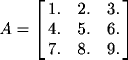
is singular in exact arithmetic, but on Altix systems, DGETRF returns
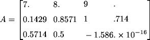
where IPIV=[3,3,3] and
info = 0. In exact arithmetic, A(3,3)
would have been 0, but roundoff error has made this entry  instead. The reciprocal condition number computed by
DGECON is
instead. The reciprocal condition number computed by
DGECON is  , which is less than the machine epsilon of
  . Therefore, DGESVX returns
info= 4 and does not try to solve any systems with this
A.
. Therefore, DGESVX returns
info= 4 and does not try to solve any systems with this
A.
You can use the condition number
to compute a simple bound on the relative error in the computed solution
to a system of equations  (see Introduction to Matrix Computations
, by Stewart). If x is the exact
solution and
(see Introduction to Matrix Computations
, by Stewart). If x is the exact
solution and  is the computed solution, let r
be the residual
is the computed solution, let r
be the residual  . If A is nonsingular:

and

From Equation 3-33 we can already see that if  is large, then the error in
  may be significantly greater than the residual
r.
may be significantly greater than the residual
r.
Since  , it follows that
  , therefore

Define the condition number  . This gives the bound
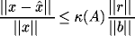
For a description of a more precise error bound based on a component-wise error analysis, see “Error Bounds”.
Another application of the condition number is to consider the computed
solution  to be the exact solution of a slightly perturbed linear
system:
to be the exact solution of a slightly perturbed linear
system:

where ΔA is small in norm with
respect to A, and Δb
is small in norm with respect to b. For Gaussian
elimination with partial pivoting, it has been shown that  and
and  , where ω is the product of ε and a slowly
growing function of n (see The Algebraic
Eigenvalue Problem, by Wilkinson). Proving that an algorithm
has this property is the stuff of backward error analysis, and it ensures
that, if the problem is well-conditioned, the computed solution is near
the exact solution of the original problem. Because
, where ω is the product of ε and a slowly
growing function of n (see The Algebraic
Eigenvalue Problem, by Wilkinson). Proving that an algorithm
has this property is the stuff of backward error analysis, and it ensures
that, if the problem is well-conditioned, the computed solution is near
the exact solution of the original problem. Because  (Equation 3-34) simplifies to

Assuming A is nonsingular,

Taking norms and dividing by ∥x∥,

Using the inequality  ,
,

and substituting  ,
,
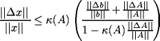
provided  . In terms of the relative backward error
  ,
,
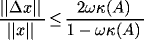
In “Error Bounds”, the backward error is defined slightly differently to obtain a component-wise error bound.
The condition number defined in the last section is sensitive to the scaling of A. For example, the matrix
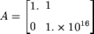
has as its inverse
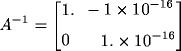
and so RCOND= . If this value of RCOND is less
than the machine epsilon on a system, DGESVX (with
FACT = `N') does not try to solve a system with this matrix.
However, A has elements that vary widely in
magnitude, so the bounds on the relative error in the solution may be
pessimistic. For example, if the right-hand side in
. If this value of RCOND is less
than the machine epsilon on a system, DGESVX (with
FACT = `N') does not try to solve a system with this matrix.
However, A has elements that vary widely in
magnitude, so the bounds on the relative error in the solution may be
pessimistic. For example, if the right-hand side in  is the following:
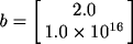
DGETRF followed by DGETRS
produces the exact answer,  .
.
You can improve the condition of this example by a simple row scaling. Scaling a problem before computing its solution is known as equilibration, and it is an option to some of the expert driver routines (those for general or positive definite matrices). Enabling equilibration does not necessarily mean it will be done; the driver routine will choose to do row scaling, column scaling, both row and column scaling, or no scaling, depending on the input data. The usage of this option is as follows:
      CALL DGESVX('E', 'N', N, NRHS, A, LDA, AF,
$         LDAF, IPIV, EQUED, R, C, B, LDB, X, LDX,
$ RCOND, FERR, BERR, WORK, IWORK, INFO) |
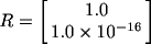
The 'E' in the first argument enables equilibration. For this example, EQUED = 'R' on return, indicating that only row scaling was done, and the vector R contains the scaling constants:
The form of the equilibrated problem is:

or  , where
  is returned in A:

and  is returned in B:

The factored form, AF, returns the same matrix
as A in this example, because
A is upper triangular, and RCOND = 0.3,
which is the estimated reciprocal condition number for the equilibrated
matrix. The only output quantity that pertains to the original problem
before equilibration is the solution matrix X.
In this example, X is also the solution to
the equilibrated problem because no column scaling was done, but if
EQUED had returned 'C' or 'B'
and the solution to the equilibrated system were desired, it could be
computed from  .
.
Iterative refinement in LAPACK uses all same-precision arithmetic, a recent innovation, because it was long believed that a successful algorithm would require the residual to be computed in double precision. The following example illustrates the results of iterative refinement; “Error Bounds”, discusses the error bounds computed in the course of the algorithm.
One possible use of iterative refinement is to smooth out numerical differences between floating-point number representations. For example, a result computed on a system, which has about 13 digits of accuracy, may be improved on IEEE system, which has about 15 digits of accuracy, through the 0(n2) process of iterative refinement, instead of the 0(n3) process of recomputing the solution.
The classic
example of an ill-conditioned matrix is the Hilbert matrix, defined by  . For example, the 5-by-5 Hilbert matrix is
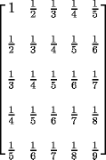
which has a condition number of  . A rule of thumb (“Condition Estimation”)
suggests almost 8 digits of accuracy in the solution are possible on systems,
because
. A rule of thumb (“Condition Estimation”)
suggests almost 8 digits of accuracy in the solution are possible on systems,
because  and
and  . If the matrix is factored using DGETRF
and DGETRS is used to solve
. If the matrix is factored using DGETRF
and DGETRS is used to solve  , where
  .
.
In
addition to performing iterative refinement on each column of the solution
matrix, DGERFS and the other
xxxRFS routines also compute error bounds for
each column of the solution. These bounds are returned in the real arrays
FERR (forward error) and BERR (backward error),
both of length NRHS. For a computed solution
x^ to the system of equations  , the forward error bound ƒ is the following:

and the backward error bound ω bounds the relative errors in each component of A and b in the perturbed equation 2 from “Use in Error Bounds”.

In Example 3-5, the first column of the inverse of
the Hilbert matrix of order 5 is computed by solving  , and DGERFS computed error bounds
of
, and DGERFS computed error bounds
of  and
and  on systems. This provides direct information about
the solution; its relative error is at most 0(10-8
); therefore, the largest components of the solution should
exhibit about 8 digits of accuracy, and the system for which this solution
is an exact solution is within a factor of epsilon
on systems. This provides direct information about
the solution; its relative error is at most 0(10-8
); therefore, the largest components of the solution should
exhibit about 8 digits of accuracy, and the system for which this solution
is an exact solution is within a factor of epsilon  from the system whose solution was attempted, so the
solution is as good as the data warrants.
from the system whose solution was attempted, so the
solution is as good as the data warrants.
The component-wise relative backward error bound (equation 3) is
more restrictive than the classical backward error bound  , because it assumes
  has the same sparsity structure as
  , because if
  is 0, so must be
  . The backward error for the solution x^
is computed from the equation
. The backward error for the solution x^
is computed from the equation
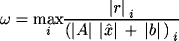
where  , and the forward error bound is computed from the equation

where γ is the maximum number of nonzeros in any row of
A. To avoid computing A
-1 an approximation is used for  , where g is the nonnegative
vector in parentheses (see Arioli, et al., for details).
, where g is the nonnegative
vector in parentheses (see Arioli, et al., for details).
Subroutines to compute
a matrix inverse are provided in LAPACK, but they are not used in the
driver routines. The inverse routines sometimes use extra workspace and
always require more operations than the solve routines. For example, if
there is one right-hand side in the equation  , where A is a square general
matrix, the solves following the factorization require 2
n2 operations, while inverting
the matrix A requires 4/3n
3 operations, plus another 2n
2 to multiply b by
A-1. The inverse must be
computed only once, however, and the cost can be amortized over the number
of right-hand sides. Because multiplying by the inverse may be more efficient
than doing a triangular solve, the extra cost to compute the inverse may
be overcome if the number of right-hand sides is large.
, where A is a square general
matrix, the solves following the factorization require 2
n2 operations, while inverting
the matrix A requires 4/3n
3 operations, plus another 2n
2 to multiply b by
A-1. The inverse must be
computed only once, however, and the cost can be amortized over the number
of right-hand sides. Because multiplying by the inverse may be more efficient
than doing a triangular solve, the extra cost to compute the inverse may
be overcome if the number of right-hand sides is large.
In some applications, the best solution
to a system of equations  that does not have a unique solution is required. If
A is overdetermined, that is, A
is
that does not have a unique solution is required. If
A is overdetermined, that is, A
is  with
with  and rank at least n, the
system does not have a solution, but the linear least squares problem
may have to be solved:
and rank at least n, the
system does not have a solution, but the linear least squares problem
may have to be solved:

If
A is underdetermined, that is, A
is  with
with  , generally many solutions exist, and you may want to
find the solution X with minimum 2-norm. Solving
these problems requires that you first obtain a basis for the range of
A, and several orthogonal factorization routines are provided
in LAPACK for this purpose.
, generally many solutions exist, and you may want to
find the solution X with minimum 2-norm. Solving
these problems requires that you first obtain a basis for the range of
A, and several orthogonal factorization routines are provided
in LAPACK for this purpose.
An orthogonal factorization decomposes a general  matrix A into a product of
an orthogonal matrix Q and a triangular or
trapezoidal matrix. A real matrix Q is orthogonal
if
matrix A into a product of
an orthogonal matrix Q and a triangular or
trapezoidal matrix. A real matrix Q is orthogonal
if  , and a complex matrix Q is
unitary if
, and a complex matrix Q is
unitary if  . The key property of orthogonal matrices for least squares
problems is that multiplying a vector by an orthogonal matrix does not
change its 2-norm, because
. The key property of orthogonal matrices for least squares
problems is that multiplying a vector by an orthogonal matrix does not
change its 2-norm, because

LAPACK provides four different orthogonal factorizations for each data type. For real data, they are as follows:
DGELQF: LQ factorization
DGEQLF: QL factorization
DGEQRF: QR factorization
DGERQF: RQ factorization
Each of these factorizations can be done regardless of whether
m or n is larger, but the
QR and QL factorizations are
most often used when  , and the LQ and
RQ factorizations are most often used when
, and the LQ and
RQ factorizations are most often used when  .
.
The
QR factorization of an m-by-
n matrix A for  has the form

where Q is an m-by- m orthogonal matrix, and R is an n-by-n upper triangular matrix. If m > n, it is convenient to write the factorization as
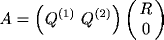
or simply

where  consists of the first n columns
of Q, and
consists of the first n columns
of Q, and  consists of the remaining m-
n columns. The LAPACK routine SGEQRF
computes this factorization. See the
LAPACK User's Guide for details.
consists of the remaining m-
n columns. The LAPACK routine SGEQRF
computes this factorization. See the
LAPACK User's Guide for details.
Example 3-6. Orthogonal factorization
The result of calling DGEQRF with the matrix A equal to
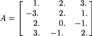
is a compact representation of Q and R consisting of
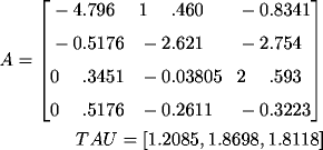
The matrix R appears in the upper triangle of A explicitly:
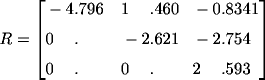
while the matrix Q is stored in a factored
form  where each
  is an elementary Householder transformation of the following
form:
is an elementary Householder transformation of the following
form:  . Each vector
  has
has  and
and  is stored below the diagonal in the
  column of A. Therefore,
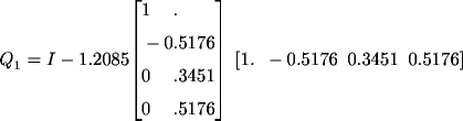
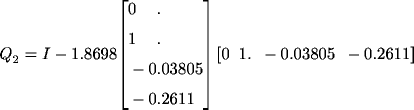
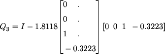
Each
transformation is orthogonal (to machine precision) because τ is chosen
to have the value  , so that

In the example of the last subsection, the elementary orthogonal matrices Qi were expressed in terms of the scalar τ and the vector v that defines them, without multiplying out the expression. This was done to make the point that the elementary transformation is most often used in its factored form. This subsection describes one application in which multiplication by the orthogonal matrix Q is required. An alternative interface for this application is the LAPACK driver routine DGELS.
Given the QR factorization of a  matrix A with
m>n (Equation 3-57),
if R has rank n,
the solution to the linear least squares problem (Equation 3-55)
is obtained by the following steps:
matrix A with
m>n (Equation 3-57),
if R has rank n,
the solution to the linear least squares problem (Equation 3-55)
is obtained by the following steps:
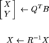
The LAPACK routine DORMQR is used in step 1 to multiply the right-hand side matrix by the transpose of the orthogonal matrix Q, using Q in its factored form. The triangular system solution in step 2 can be done using the LAPACK routine DTRTRS.
Continuing the example of “Orthogonal Factorizations”,
suppose the right-hand side vector is  . Multiplying b by
  by using the LAPACK routine DORMQR,
you get
by using the LAPACK routine DORMQR,
you get
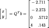
and after solving the triangular system with the 3-by-3 matrix R,

The last m-n
elements of  can be used to compute the 2-norm of the residual, because
  . Here,
  .
.
The DORMxx routines described in the previous subsection are useful for operating with the orthogonal matrix Q in its factored form, but sometimes it is the matrix Q itself that is of interest.
For example, the first step in the computational procedure for the
generalized eigenvalue problem  is to find orthogonal matrices U
and Z such that
is to find orthogonal matrices U
and Z such that  is upper Hessenberg and
  is upper triangular (see Golub and Van Loan for details).
First, the matrix B is reduced to upper triangular
form by the QR factorization, and
A is overwritten by
is upper triangular (see Golub and Van Loan for details).
First, the matrix B is reduced to upper triangular
form by the QR factorization, and
A is overwritten by  , using the subroutines of the previous section for multiplying
by the orthogonal matrix.
, using the subroutines of the previous section for multiplying
by the orthogonal matrix.
Next, the updated A is reduced to Hessenberg
form while preserving the triangular structure of B
by applying Givens rotations to A and
B, alternately from the left and the right. In order to
obtain the orthogonal matrices U and
Z that reduce the original problem, it is necessary to keep
a copy of the matrix Q from  and continually update it. This requires that
Q be generated after the QR factorization.
and continually update it. This requires that
Q be generated after the QR factorization.
The DORGxx routines generate the orthogonal matrix Q as a full matrix by expanding its factored form. Using the example of “Orthogonal Factorizations”, Q can be generated from its factored form by using the following Fortran code:
DO J = 1, N
   DO I = J+1, M
      Q(I,J) = A(I,J)
   END DO
END DO
CALL GORGQR(M,M,N,Q,LDQ,TAU,WORK,LWORK,INFO) |
where the data from the QR factorization of A has been copied into a separate matrix Q because DORGQR overwrites its input data with the expanded matrix. The orthogonal matrix is returned in Q:
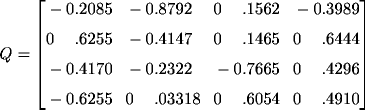
The matrix Q(1), consisting of only the first n columns of Q, could be generated by specifying N, rather than M, as the second argument in the call to DORGQR.
The results obtained by LAPACK routines should be deterministic; that is, if the same input is provided to the same subroutine in the same system environment, the output should be the same. However, because all computers operate in finite-precision arithmetic, a different order of operations may produce a different set of rounding errors, so results of the same operation obtained from different subroutines, or from the same subroutine with different numbers of processors, are not guaranteed to agree to the last decimal place.
In testing LAPACK, the test ratios in the following table were used
to verify the correctness of different operations. All of these ratios
give a measure of relative error. Residual tests are scaled by 1/ε,
the reciprocal of the machine precision, to make the test ratios
O(1), and results that are sensitive to conditioning are
scaled by 1/κ, where  is the condition number of the matrix
A, as computed from the norms of A
and its computed inverse A-1
. If a given result has a test ratio less than 30, it is
judged to be as accurate as the machine precision and the conditioning
of the problem will allow. See the Installation Guide for LAPACK
for further details on the testing strategy used for LAPACK.
is the condition number of the matrix
A, as computed from the norms of A
and its computed inverse A-1
. If a given result has a test ratio less than 30, it is
judged to be as accurate as the machine precision and the conditioning
of the problem will allow. See the Installation Guide for LAPACK
for further details on the testing strategy used for LAPACK.
Table 3-2. Verification tests for LAPACK (all should be O (1))
Operation or result | Test ratio |
|---|---|
Factorization A = LU |
|
Solution x^ to Ax = b |
|
Compared to exact soln x |
|
Reciprocal condition number RCOND | max(RCOND, κ)/min( RCOND, κ) |
Forward error bound f |
|
Backward error bound ω | ω/ε |
Computation a A-1 |
|
Orthogonality check for Q |
|
ε = Machine epsilon n = Order of matrices κ = | |






