BDSpro requires that IRIX version 6.2 (or higher) and NFS (version 2.0 or 3.0) are installed on client and server systems. It also requires that the applications that use BDSpro services perform page-aligned I/O and direct reads and writes (see “How BDS Works” in Chapter 1).

BDSpro software must be installed on both client and server systems. See the BDSpro Release Notes for instructions on software installation.

Silicon Graphics currently ships SCSI disks manufactured by Quantum and IBM. Quantum disks excel in random access and relatively small I/O operations, and IBM disks excel in large sequential access operations. Because of the operating characteristics of BDS, disks that excel in large sequential access operations offer better performance and are therefore a better choice.

Most BDS installations are likely to use fast-and-wide SCSI controllers with speeds of 20 MB per second. The IBM drives provided by SGI spin at about 7 MB per second on the outer zone and 5 MB per second on the inner zone. If we assume a transfer rate of 5 MB per second, it is apparent that 4 drives will completely saturate a single 20 MB per second controller.

Silicon Graphics provides SCSI boxes with an eight-drive capacity that are configured for one SCSI channel. Since channel speed is 20 MB per second and drive speed is approximately 5 MB per second, eight drives offer more bandwidth than is needed. Therefore it is possible to configure SCSI boxes with two SCSI channels per box, doubling the bandwidth for each box.

For maximum sequential performance with the minimum number of disks, purchase more controllers and use one controller for every four disks.

BDSpro performance is highly dependent on the local performance of XFS on the server system. In general, BDSpro requires a local XFS access speed that is twice as high as the speed at which BDSpro is to perform. For example, if BDSpro is to operate at a rate of 50 MB per second, the server XFS rate must be at least 100 MB per second. This XFS rate is required to offset the overhead that BDSpro protocols impose on network transactions.

To measure local XFS performance, use lmdd commands similar to those shown below.

This command creates testfile, a 500 MB file with a blocksize of 7 MB:

server# lmdd of=/export/bds/testfile bs=7m move=500m direct=1
497.00 MB in 5.83 secs, 85.29 MB/sec

This command performs a direct read on testfile with a transfer size 7 MB; the output shows the XFS transfer rate:

server# lmdd if=/export/bds/testfile bs=7m move=500m direct=1
497.00 MB in 4.44 secs, 111.92 MB/sec

Inadequate XFS performance can frequently be corrected by properly configuring disks and by setting the correct size for direct memory access operations. These topics are explained in the sections that follow.

Configuring Disks for BDSpro

XFS uses a logical volume manager, xlv, to stripe data across multiple disk drives. On striped disks, large XFS requests are split and sent to each disk in parallel. The high sequential performance of XFS is attributable to this parallelism. (See Chapter 7 of IRIX Admin: Disks and Filesystems for more information.)

The size of data transfers is an important consideration in planning logical volumes. For example, assume that a logical volume contains 10 disks and the track size is 64 KB. In this case, transfers of 640 KB or larger are required to get all drives running simultaneously. If the data transfer size is 320 KB, only five drives are active in an I/O operation. Because only half of the available disks are used, a transfer size of 320 KB is very inefficient, reducing the total performance by half. With proper striping of logical volumes, however, disk performance can be maximized.

Understanding Logical Volume Stripping

The xlv_make utility is used to stripe the disks in a logical volume. By default, xlv_make divides the disk into tracks and uses one track from each disk in rotation to create a stripe. The amount of data that xlv_make allocates on a single drive before going to the next is called the stripe unit. The stripe unit and the number of disks in the logical volume determine the stripe width, or

stripe width = stripe unit × number of disks

Figure 2-1 illustrates a logical volume containing four disks. Notice from this figure that the stripe unit is set to two tracks instead of one (the default stripe unit size). If we assume a track size of 100 KB (track size is set by disk manufacturers), the stripe width for this logical volume is 800 KB.

Figure 2-1. Effects of the Stripe Unit and Disk Number on Stripe Width

Determining the Size of Stripe Units

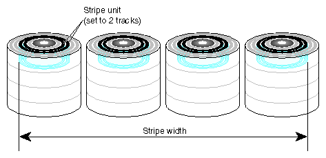
When you create a logical volume, you can specify a stripe size using the stripe_unit argument of xlv_make (see the xlv_make(1M) reference page). Specifying the proper size of the stripe unit is the key to optimizing I/O performance. In most cases, the objective in setting the stripe_unit is to achieve a particular bandwidth; but you might also need to adjust the stripe size to accommodate an application that uses a fixed transfer size.

The transfer size should be a multiple of the system's page size. The transfer size should also be a multiple of the stripe width (800 KB in Figure 2-1). If the application needs the bandwidth of all four disks but is reading with a transfer size of 400 KB, you could set the stripe unit to one track instead of two to achieve the required bandwidth with half the transfer size.

Optimizing the Stripe Unit Size

It is not always advisable to use the smallest possible stripe unit. While small requests can be effective with read transfers because of the read-ahead assistance that SCSI track buffers offer, small stripe units degrade write performance.

For example, consider what happens when data is written using the default stripe unit size of one track. The write is broken into tracks and each track is sent to a different disk. When the data arrives at the controller, the controller first waits for the disk head to move to the beginning of the track before it writes the data. This wait, commonly referred to as a rotational delay, occurs between each track that is written to the same disk; as a result, using a one-track stripe unit reduces the write performance to half of the read performance.

It is possible to achieve higher write performance by using larger stripe units. Table 2-1 shows the effects of increasing the size of stripe units on XFS write performance.

Table 2-1. Effects of Stripe Unit Size on XFS Write Performance

Stripe Unit	Request Size	Write Performance
1 track = 100 KB[a]	1 track × 4 disks = 400 KB	1/2 read performance
2 tracks = 200 KB	2 tracks × 4 disk = 800 KB	2/3 read performance
3 tracks = 300 KB	3 tracks × 4 disks = 1.2 MB	3/4 read performance
4 tracks = 400 KB	4 tracks × 4 disks = 1.6 MB	4/5 read performance
[a] Default size used by the xlv_make command.

Table 2-2 shows the performance for BDSpro (version 1.0) using IBM drives with a 2 GB capacity and a HIPPI network. Three disks were configured on each controller; the transfer size was set to the stripe width size. Notice from Table 2-2 that BDS writes are slower than XFS writes. This is due to the synchronous nature of BDS write operations.